Intro to RNASeq (Lecture)
Last Updated: 2020-03-03
Last Delivered: 2019-11-05
Google Slide Deck
You can view the latest version of the Google Slides deck at this link.
Part 0: Introduction
Slide Deck
View the slide deck for this tutorial. The webpage will contain more detailed information than the slide deck, and is written to have more references to related information.
0.1 Formatting in This Document
Throughout this tutorial, there will be formatting cues to highlight various pieces of information.
This is a warning. Common pitfalls, cautionary information, and important points to consider will appear like this.
File contents or literal values will appear like this. We will use this format
to illustrate file formats.
0.2: Goals
- Learn how RNASeq techniques can be applied to your research program
- Learn basic experimental designs for RNASeq projects
- Become familiar with core file formats of genomics
0.3: Scope of the Tutorial
This tutorial has a lecture format and will cover the principles and concepts that underlie RNASeq experimental design and data analysis. This tutorial will not cover the mechanistic details of how to analyze RNASeq data - that will be covered in the companion hands-on tutorial.
Part 1: RNASeq Overview
1.1: What is RNASeq?
RNASeq is a technique that uses high-throughput sequencing technologies to assay the transcriptome, or the transcribed portions of a genome. Which parts of the genome are transcribed depends on many factors, including biotic or abiotic stressors, organ or tissue type, developmental stage, and genotype of the samples. However, the transcriptome size is much smaller than the genome size, which allows researchers to sample many more individuals with a limited budget. RNASeq data can be used to assemble transcript sequences, detect alternative splicing events, or test for differential expression across a set of conditions. Because RNASeq data is sequence-based, it can even be used to identify genetic polymorphisms, with the caveat that they will only be found in highly-expressed regions of the genome.
Relatively new sample handling library preparation protocols allow researchers to tag sequencing reads as originating from the RNA of a single cell (single-cell RNASeq, scRNASeq). This allows researchers to study expression at very fine-grained resolution. Single-cell RNASeq requires special considerations, both in terms of analysis and wet-bench molecular techniques, and we will not cover it in high detail here.
“Typical” RNASeq protocols involve extraction of RNA from groups of cells that are homogenized, or bulked. It is broadly labeled as bulk RNASeq to distinguish it from scRNASeq. Most of the material we will cover in this tutorial will cover either general experimental design or bulk RNASeq handling.
1.2: RNASeq vs. Other Genomics Technologies
Because RNASeq targets transcribed, or expressed, parts of the genome, its most direct comparisons are to other expression-focused genomics technologies.
In comparison to expression microarrays, RNASeq has higher dynamic range and does not depend on a designed assay, which means that it potentially has higher sensitivity and is easier to apply to systems which are not genomics model systems. However, the analytical framework in place for analyzing microarray data is more mature and standardized, meaning that RNASeq studies may have lower repeatability than those based on microarrays. RNASeq analysis is becoming more standardized, however, and a strong grounding in experimental design can allow researchers to account for bias and experimental error in their analysis. RNASeq also allows single-nucleotide resolution, which means that the data can be used to discover variants as well as expression differences.
In comparison to EST (expressed sequence tag) sequencing, RNASeq is much faster and cheaper per nucleotide of data. EST sequencing does not rely on a reference genome sequence, but is much lower throughput. EST sequencing also does not yield any information about the relative expression levels of various transcripts, so it precludes differential expression analysis.
RNASeq is relatively affordable, has high sensitivity to detect expression differences, can be used to detect isoforms and genetic variants, but has high noise and can suffer from low repeatability. However, like scientific research in general, careful experimental design can mitigate the repeatability problems.
1.3: Typical RNASeq Workflow
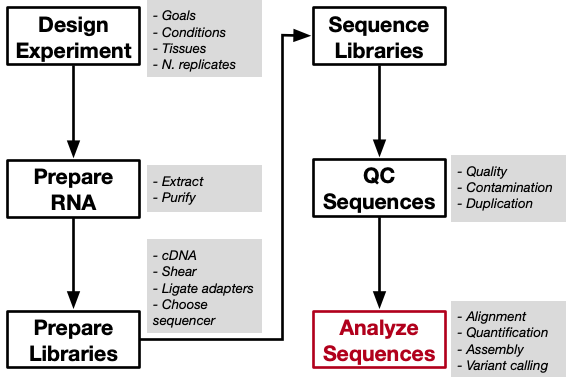
The typical RNASeq workflow follows the diagram shown below. The number of samples and the setup of the actual experimental treatments will depend on the goals of the project.
Part 2: RNASeq Experimental Considerations
Designing an RNASeq experiment draws upon the same principles of general experimental design. In principle, the expression values of the genes that are assayed by RNASeq technologies are phenotypes that are being measured by the researcher. Randomization, replication, and blocking are all important components of an RNASeq experiment, and should be included where logistically (and financially) possible.
It is important to distinguish between a biological replicate and a technical replicate. A biological replicate is used to assay variation in the biological material that is being studied. For example, a study that is designed to test the effects of a drug on gene expression in a mouse model may treat six mice each with saline and a dose of the drug. The experiment would have six biological replicates per treatment. If each mouse in this experiment then had two separate RNA extractions, library preparations, and sequencing runs, then there would be two technical replicates for each mouse. The total size of the experiment would be 24 sequencing runs, or 2 treatments * 6 biological replicates per treatment * 2 technical replicates per biological replicate.
Technical replicates are not always nested within biological replicates, but are collected to assay the degree of variation in the technique or data collection aspect of the experiment. Technical variation is generally much lower than biological variation, but this is not universally true, and it is good practice to include both biological and technical replicates in your experimental designs, when possible.
Your experiment should also include randomization to remove biases between the blocking factors of your experiment. For example, it is possible to only perform a certain number of extractions in a single day. The samples that are extracted on each day should be randomized with respect to the experimental condition, such that the “extraction day” effect is not perfectly confounded with the experimental treatment effect.
2.1: Experimental Design
The exact design of an RNASeq experiment will depend on the researcher’s goals. For example, for transcriptome assembly, a researcher may want to sample several replicates each from multiple tissues of an organism and sequence them to high depth. For differential gene expression analysis, a design that samples a single tissue from multiple biological replicates within each treatment is more appropriate.
The sections that follow will have brief overviews of common experimental designs in RNASeq projects. More complicated designs are possible, with high degrees of replication across hierarchical categorical variables, such as with agricultural experiments, but most budgets do not allow for such intense data collection via RNASeq.
Pairwise Two-Group Comparison
This is a very simple design that is used to test the effect of a single factor, such as a drug compound or a single stress condition.
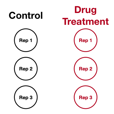
In this example, the black samples represent the control condition and the red samples represent the treatment condition. There are several biological replicates per condition, which usually means different individuals of the same strain or genotype that were subjected to the same treatment.
Factorial Design
This design is slightly more complicated and is used to test for the effect of interaction between two experimental variables. For example, the effects of both heat stress and salt stress on plant gene expression.
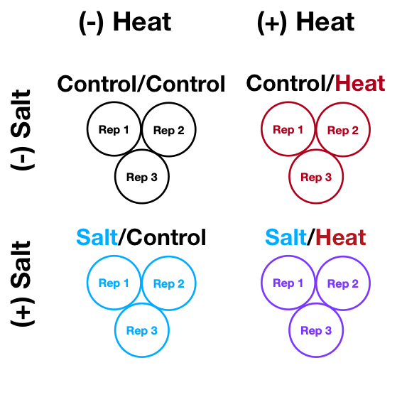
In this example, the black circles are the control group, having received neither heat nor salt treatment. The blue circles have been subjected to the salt treatment, but not the heat treatment. The red circles were treated with heat, but not salt. The violet circles are samples that were treated with both heat and salt.
This design allows the researcher to isolate both the effects of heat stress and salt stress on gene expression, and includes a group for testing the interaction between heat and salt.
Also note that the physical arrangement of these samples in the experimental area (lab/field/greenhouse/growth chamber/cage/tank/etc) should be randomized, if possible.
Nested Design
This design is related to the factorial design in that it stratifies the effects of experimental variables and nests them in a hierarchy. However, unlike a factorial design, some combinations of factors cannot be tested. For example, a researcher may be interested in the effects of heat stress in three different populations of a plant sampled from across its range. This is a nested and not a factorial design because there cannot be replication of the individuals in the experiment, i.e., exactly one individual can get exactly one treatment. In the factorial design, it is assumed that the individuals are similar enough such that they can be replicated in different experimental conditions.
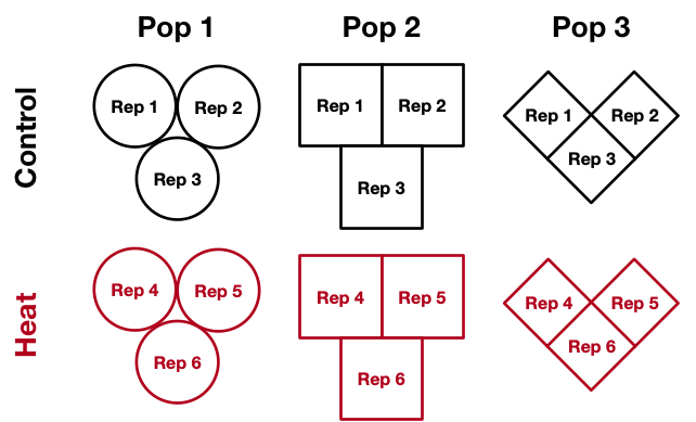
This type of design is common in ecological experiments, where the samples simply cannot be replicated across treatments.
Matched Pair Design
This design is only applicable when there are exactly two treatments that are to be compared and the individuals in the experiment can be grouped into pairs. For example, a researcher may be interested in the effect of a compound on two different tissues from the same patient, or the effect of a drug on cancerous and non-cancerous tissue from the same person.
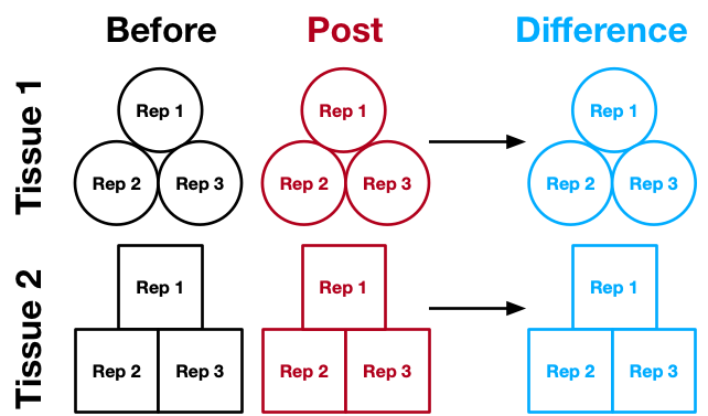
In these simple illustrations, we are assuming that the variation between replicates in the same treatment is small relative to the variation among conditions. This is generally regarded to be true for experimentally convenient organisms, such as clones of culturable microbes, genetic stocks of research animals, and inbred lines or doubled haploid plants. For wild-caught samples or human subjects/patients, this is not true, and variation among individuals must be taken into effect. The individual used in the study would then be treated as a random effect*.
In the examples above, we are interested in the effects of the specific experimental conditions that are being tested, and we have sampled all of the levels of interest, so we treat them as fixed effects.
*: The exact definition of what is a fixed effect and what is a random effect varies by discipline. We cannot include a rigorous discussion of all definitions that are in common use, but one aspect that is common to each is that random effects are assumed to be uncorrelated with the treatments and fixed effects are assumed to be correlated with the treatments.
2.2: Molecular Biology Techniques
The experimental design principles mentioned in the previous section will help to decide the number of biological samples that will be used in your projects. There are, however, additional concerns that relate to the handling of the material once it has been harvested from your experiment. These relate to the type of library preparation protocol and sequencing technology that you choose for your data collection.
Short-Read Library Preparation
Library preparation is the step at which the extracted RNA is prepared for sequencing. We will focus on short-read protocols in this document, but later sections will touch on long-read sequencing.
The library preparation step is where you determine several important parameters about your data set:
- Paired-end or single-read sequencing
- Insert size (if paired end)
- Strand specificity
Paired-end reads are more expensive to collect, but yield much more information than single-read sequencing. The technology is such that the reads have a pre-determined relative orientation and are derived from a physical molecule of a certain size, so they more easily map to unique regions of the genome.
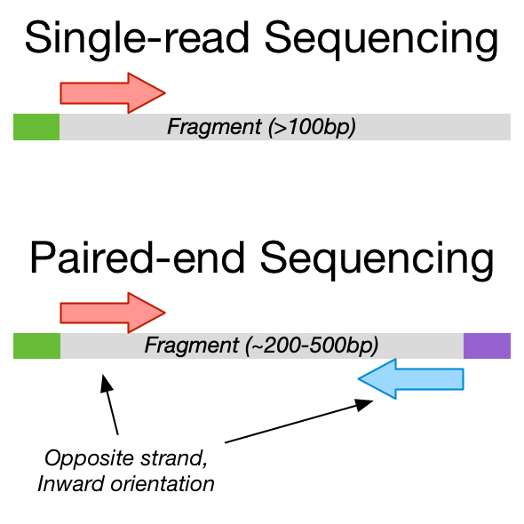
In the above cartoon, the green and purple pieces are the sequencing adapters.
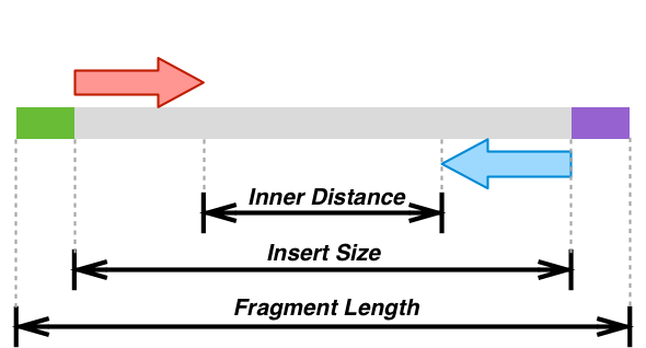
The insert size consideration is only applicable for paired-end data. Library preparation involves shearing or fragmenting the isolated RNA into fragments that are approximately the same size before ligating the sequencing adapters. The diagram above, the known physical distance between the reads is directly related to the insert size. If the organism you are studying tends to have short genes, then a shorter insert size will yield higher coverage of the transcripts. If the organism tends to have longer genes, then a long insert size will give more information about the exons from which the reads were derived.
Various genomics tools and protocols may require you to know the mean and variance in one of the lengths shown below. It is important to know the difference because the terms have names that are easily confused.
Strand-specific libraries increase the accuracy of assaying the expression level of any given gene. A strand-specific library ensures that reads are derived from only one of the sense or antisense strand. That is, reads map either to the same or opposite strand of the gene sequence on the genome, not both. The directionality of the read is taken into account during expression counting, reducing the error and uncertainty of how many reads are derived from intact transcripts. It also allows resolution of genes that share base positions in the genome, but are on different strands. This happens more frequently in prokaryotes and microbial eukaryotes with compact genomes than in organisms with very large and/or polyploid genomes.
The default protocol that the University of Minnesota Genomics Center (UMGC) uses for short-read RNASeq applications is the Illumina TruSeq stranded mRNA kit. This produces a reversely-stranded paired-end library.
2.3: How Much Sequence Data to Collect
For differential gene expression analyses in most animals or plants, we recommend a minimum of 20 million reads per sample. For simpler eukaryotes (e.g., nematodes or yeast), 10 million reads per sample may suffice. You should have at least three biological replicates (i.e., samples from three different individuals or clonal pools) per experimental condition, if possible. There are cases where three replicates is excessive, such as high-resolution time series analyses, so use your best judgment.
The UMGC recommends 50bp paired-end sequencing technology for differential gene expression analysis. For isoform-level expression or alternative splicing analysis, they recommend at least 125bp paired-end technology. It is possible to use single reads for differential gene expression, but it is not a widely requested technology, and it may take longer to move through the queue.
The ENCODE project maintains guidelines for RNASeq experiments that may be helpful. You may also refer to this page from Genohub that lists recommendations for coverage for a variety of applications.
2.4: Metadata (KEEP NOTES!)
Keeping notes on your experiments, both at the organism collection or rearing stage, and at the molecular genetics lab bench stage, is critical. Experimental factors, such as cages/plots/plates in which the experimental organisms are reared can be large sources of variation that reduce power in your experiment if they are not properly accounted for. Similarly, the storage and handling conditions of the material, the day of RNA extraction, the day of library preparation, lane or flowcell of sequencing instrument, and the technician who performed the protocols can all introduce bias to your results. You should randomize across these experimental factors whenever possible, and keep detailed notes on them.
For example, collaborative work between UMGC and MSI analysts has demonstrated that sample storage conditions (RNAlater storage and liquid nitrogen flash-freezing and storage at -80C) have differential effects on observed gene expression in fish (Passow et al. 2018). The way samples were processed is an important piece of metadata that should be recorded and maintained with the actual data whenever possible. Unfortunately, this sort of information is not frequently deposited into public repositories, such as NCBI SRA, so exercise caution when using publicly-available datasets.
An example (but not necessarily complete!) list of metadata items to keep for your samples is
- RIN score
- RNA concentration
- Extraction protocol
- Extraction time/date
- Who performed the extractions
- Sample storage conditions
- Tissue type or treatment
- Developmental time of sample
- Bench/cage/plate/tank/region/population/etc. of sample rearing or collection
- Library preparation protocol
- Sequencing instrument ID
- Flowcell ID
- Lane number*
- Sample barcode*
*: The UMGC generally pools barcodes (samples) and splits them across all lanes on a flowcell to reduce lane-specific effects from being perfectly confounded with sample ID. However, if you have your material sequenced at a different facility, this may not be the case. Keep track of this information!
Ideally, you would also make this metadata available when you publish your dataset. This greatly improves reproducibility and aids in analyzing datasets from multiple sources.
Part 3: Analytical Workflow and File Formats
This section will deal more specifically with what the analytical side of RNASeq projects look like. We will not be covering how to do the analyses in detail in this section, but we will cover what the overall analysis strategy is and what file formats are involved.
3.1: Overall Workflows
The overall workflow of RNASeq analysis will depend on your goals: a workflow for transcriptome assembly will look slightly different from a workflow for differential gene expression analysis. We will sketch workflows for common types of RNASeq analysis below. Depending on the idiosyncrasies of your data and research system, your workflow may deviate slightly from the sketches we show below.
Differential Gene Expression (DGE) Analysis
The goal of this type of analysis is to identify genes that significantly change in expression level in response to some condition or treatment. It generally requires at least three biological replicates per condition. This includes combinations of conditions if you are testing in a factorial experiment.
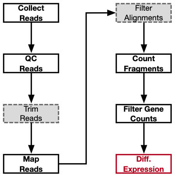
The steps shown in grey dashed boxes are optional, but generally recommended.
In this analysis, you are testing that the expression level of a gene is significantly different between treatments or conditions, using read counts as a proxy for expression level. The variation in read counts among biological replicates serves as the sample variance against which you test the differences in expression. The list of genes that are differentially expressed may then be used to generate more focused hypotheses. For example, the list of differentially expressed genes may be used as a candidate list for validation in a follow-up experiment with a more targeted assay of gene expression like qRT-PCR, or knock-out and phenotypic assays.
We will be covering this workflow in the hands-on portion of the tutorial.
Transcriptome Assembly
The goal of this type of project is to generate a set of reference transcript sequences for the organism or tissue of interest. Inclusion of biological variation (i.e., sampling of multiple tissues, developmental time points, or stress conditions) increases the usefulness of the assembly by “capturing” more expressed sequences. Not all transcripts are expressed at all times or under all conditions.
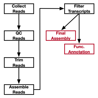
Note that in this workflow, the read trimming is required. Contamination with sequencing adapters will cause non-biological sequence to be incorporated into your reference assembly, and my cause erroneous chimeric transcripts to be assembled (by linking disparate transcripts with identical non-biological sequence). This is not as much of an issue with differential gene expression analyses because read mapping tools can mask sequence that does not match the reference genome. Further, the transcriptome assembly should be filtered to remove biological contaminant sequences. There is often contamination from non-target organisms in samples, such as soil bacteria in plant samples.
Final products of a transcriptome assembly workflow are often a reference assembly and some degree of functional annotation or homologous locus information.
Variant Discovery
RNASeq data can also be used to discover genetic variants such as single nucleotide polymorphisms (SNPs) or short insertions and deletions (indels). This is mostly useful in systems that have a reference transcriptome but not a reference genome. It may also be of interest if you would like to enrich the variants for those that occur in transcribed sequences, or if you would like to identify genetic variants alongside testing for differential expression.
In systems with very high genetic diversity, iteratively identifying variants and re-mapping reads to a “corrected” reference may improve the ability to resolve expression differences by reducing mapping uncertainty and increasing the number of reads that can be matched by accounting for genetic diversity. In most model systems, however, this is not necessary.
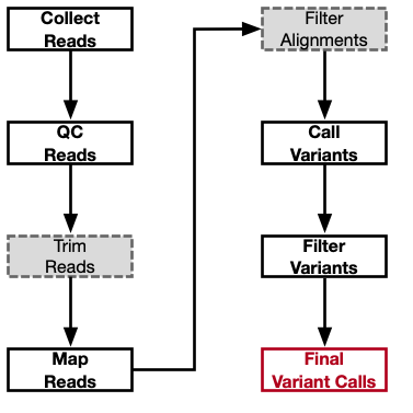
This workflow looks very similar to the differential expression workflow. However, instead of counting reads that map to gene features, you instead use sequence differences between the reads and the reference to identify genetic variants in your sample. Once variants have been identified, it is a standard practice to apply filtering on the variants based on read depth, allele frequency, heterozygosity, and call rate.
It should be noted that if you call variants from RNASeq data, they will be unrepresentative of genetic diversity on a whole-genome scale. RNASeq data is highly biased by expression level (rare transcripts have very low coverage), so you will not discover variants in rare transcripts. Due to the strong dependence of read depth on expression level, RNASeq data is also not appropriate to discover gene deletion or duplication events.
Additionally, RNASeq enriches for functional regions of the genome, which may be under purifying selection, so genetic diversity in RNASeq data may underestimate the genetic diversity genome-wide.
However, it is still useful for identifying genetic variants in experimental systems where there are very few genomic resources available.
Others
There are many other analyses that can be done with RNASeq data. Section 7 will contain brief descriptions and links to common analysis tools for the workflows described above and other, more specialized analyses.
3.2: File Formats
RNASeq is a genomics analysis, meaning it uses a suite of (mostly) standardized genomics file formats. There are some important considerations with some of the file formats, however, because they tend to have variable formats. This is a known issue in genomics, and the field is still settling on a standard way to represent some data, like gene annotation data for example.
FASTA
Holds sequence information, without any associated quality information. The
FASTA format has a sequence name, denoted with > followed by the name of the
sequence. The next line(s) have the sequences. The file may have one or more
sequence records.
>Sequence 1
ATCGA...
>Sequence 2
GGTAC...
Reference sequences are generally stored in the FASTA format.
FASTQ
Holds sequence information with associated quality scores. Each FASTQ record has
four lines: a name, a nucleotide sequence, a comment, and a quality string. The
name starts with @ and the comment starts with +. The quality scores are
stored as ASCII characters, treating each character’s decimal value as the
quality score (with a +33 offset*). You will not have to read a FASTQ
directly; the alignment programs will understand them. Quality is defined as
-log10(P that the base is called incorrectly), which is the Phred scale used in
Sanger sequencing traces.
*: Note that older FASTQ files may have a +64 offset. The most common quality control programs will auto-detect the ASCII offset and report it to you so that you will know how to tune your workflows in subsequent steps.
@D00635:256:CB8P5ANXX:1:1108:2215:2225 1:N:0:ATTACTCG+TATAGCCT
GCGCTAAAGCAGTGATTAGAGGGAAATTTATAGCACCAAATGCCCACAGAA
+
@B=BBGGGGCBDDC@GGEGGGGGGGGGGGGGFGGGEGGGGGGGGGGGGG>D
@D00635:256:CB8P5ANXX:1:1108:2547:2188 1:N:0:ATTACTCG+TATAGCCT
CCGCACATCACAAACGTGATTCTGCGAATGCTTCTGACTAGTTTTTGTCGG
+
BBBCCEGGGCGGGGGGGGGGGGCGGGGGGGGGGGGGGGGG>F>F>GGGGGG
Reads from the sequencing instrument are generally stored in the FASTQ format.
SAM/BAM
Holds alignment information. While sequence alignments can technically be stored in FASTA format, it is very inefficient for genomics datasets. Additionally, genomics alignments tend to be a series of pairwise alignments to a reference sequence, and not a multiple sequence alignment.
A SAM (Sequence Alignment/Map) file stores position, read sequence, mismatch information, and alignment confidence scores, among other information. A BAM file is a binary representation of a SAM file, which is machine-readable and much smaller on disk. You generally will not have to parse a SAM/BAM file on your own; most of the tools you will encounter will know how to perform operations on them.
@HD VN:1.6 SO:coordinate
@SQ SN:ref LN:45
r001 99   ref 7  30 8M2I4M1D3M = 37 39  TTAGATAAAGGATACTG *
r002 0    ref 9  30 3S6M1P1I4M * 0  0   AAAAGATAAGGATA    *
r003 0    ref 9  30 5S6M       * 0  0   GCCTAAGCTAA       * SA:Z:ref,29,-,6H5M,17,0;
r004 0    ref 16 30 6M14N5M    * 0  0   ATAGCTTCAGC       *
r003 2064 ref 29 17 6H5M       * 0  0   TAGGC             * SA:Z:ref,9,+,5S6M,30,1;
r001 147  ref 37 30 9M         = 7  -39 CAGCGGCAT         * NM:i:1
A link to the SAM/BAM specification is here.
GTF/GFF (GFF3)
Holds genomic feature annotations, like gene models. These formats are somewhat
loosely defined, but files from databases such as NCBI or Ensembl should be
handled well by genomics analysis programs. The information stored in a GTF or
GFF includes each feature’s boundaries, type (gene, CDS, TF binding site, etc),
strand, name, and any parent/child relationships. For example, a mRNA feature
may be the child of a gene feature, and may have several CDS and exon
children features.
The GFF and GTF specifications can be found here.
GFF and GTF files are the formats that I parse “by hand” the most often. GTF or
GFF files from different sources will often contain different information in
them, so it is important to record the source and date of your annotation file.
Additionally, different sources encode the genomic coordinates in different
ways, for example, one source may call chromosome 1 chr1 and another may just
call it 1. Chromosome ordering may also differ between sources. These
mismatches must be addressed before a given reference FASTA and GTF/GFF can be
used in an analysis. Always check for agreement!
Part 4: Long Reads
The previous sections mostly dealt with short-read technologies, however, there are several long-read protocols that work with transcript sequences. Long reads have the advantage that they can query an entire transcript at once, which allows researchers to resolve isoforms of a single gene. Further, the technologies are able to assay single molecules, which reduces the need to amplify a library (which adds bias). For transcriptome assembly, long reads greatly reduce the effort required to generate a reference transcriptome, because many reads will be complete reads of a transcript. However, the RNA extraction protocols and library preparation protocols for long-read sequencing are much more expensive and specialized.
The analytical workflows for long-read RNASeq are quite different from the ones sketched in the previous sections. To analyze these data, you will need to develop a custom workflow for your data. Pacific Biosciences maintains a landing page for their isoform sequencing protocol (“IsoSeq”) with information about the nature of the data and how to analyze it. They also maintain a wiki that gives a detailed workflow, including an example analysis.
Pacific Biosciences tools are not fully functional on MSI systems just yet. The graphical analysis portal is not compatible with our scheduler, and requires a lot of hacking to get it to work. The command line utilities mostly work. Contact help@msi.umn.edu if you need assistance with Pacific Biosciences data analysis.
Part 5: Single-cell RNASeq
Single-cell RNASeq (scRNASeq) is a technique that uses a special sample handling protocol that tags each cell in a sample with a unique barcode, and each individual transcript molecule with a unique molecular identifier (UMI). The UMI serves to uniquely identify a transcript to reduce amplification bias in library preparation. Instead of using read counts as in bulk RNASeq differential expression, UMI counts are used to measure relative expression.
scRNASeq is a useful technique for identifying cellular types in a heterogeneous mixture of cells in a tissue sample. It can be used to identify rare cell types in a sample, precisely query relationships between genes and their regulatory elements, and track the development of cell lineages.
Similar to long-read sequencing technologies, the sample handling and library preparation protocols are expensive and specialized.
Part 6: University of Minnesota Genomics Center
The University of Minnesota Genomics Center offers extraction, library preparation, and sequencing services. They also offer services for long-read technologies. Their systems are connected to MSI servers to support direct data deposit into your MSI directory.
6.1: Pricing and Instruments
- HiSeq2500, click the “Pricing” tab.
- NextSeq and NovaSeq Internal
- NextSeq and NovaSeq External
For a quote, you can contact the next-gen sequencing team UMGC by emailing next-gen@umn.edu with your desired read quantity, read length, and single/paired technology. They will prepare a quote that will be good for three months from the preparation date.
For a full description of UMGC services and pricing, please see their catalogue. Note that despite what the first page says, the prices are still current, as of November 2018. The UMGC is updating their pricing schedule, however, so prices are subject to change in the next six months.
6.2: Expected Turnaround Time
The standard turnaround time for RNASeq projects at the UMGC is 6-8 weeks, assuming the libraries pass QC and there are no complications with the reagents or the instruments. For faster turnaround, you may request to use the NextSeq, which is a single lane, rather than a shared flowcell like with the other instruments.
Part 7: Helpful Links
This section will contain a list of common software tools, manuals, and guides for performing various RNASeq analyses.
7.1: Differential Gene Expression
- HTseq - generate an expression counts matrix
- featureCounts - generate an expression counts matrix
- Manual - See section 6.2
- Publication
- EdgeR - differential expression testing
- DESeq2 - differential expression testing
- CHURP - UMN Pipeline, developed by RIS at MSI
7.2: Transcriptome Assembly
For assembly evaluation for completeness/quality:
Long-read Transcriptome Assembly
- IsoSeq 3 - Pacific Biosciences
7.3: Variant Detection
7.4: Coexpression Network Construction
- WGCNA - correlational network building from gene expression data
- petal - gene coexpression network building with RNASeq data
- Camoco - gene coexpression network building with GWAS functionality
7.5: Pathway Analysis or Functional Enrichment
These are not RNASeq analysis tools in themselves, but they are commonly used to derive insights from gene lists obtained through RNASeq analyses.
- ReactomePA - pathway analysis
- clusterProfiler - GO term enrichment and pathway analysis
- Gene Set Enrichment Analysis
7.6: Single-cell RNASeq
- Seurat - clustering and alignment of single cell RNASeq profiles
- Monocle - time course and differential expression analyses with scRNASeq
Part 8: Feedback
This tutorial document was prepared by Thomas Kono, in the RIS group at MSI. Please send feedback and comments to konox006 [at] umn.edu. You may also send tutorial delivery feedback to that address.