Introduction to Pathway Analysis
Last Updated: 2026-05-27
Last Delivered: 2026-04-14
Check out the recording of this tutorial and other MSI tutorials on our YouTube channel: https://www.youtube.com/@UofMMSI/videos
Expand all details (Useful for printing!)
Collapse all details
Part 0: Introduction
This tutorial will cover the basics of running a pathway enrichment analysis or gene set enrichment analysis. We will have both a lecture portion and a hands-on portion, with command line tools.
Please see http://z.umn.edu/ris-pathway for the latest version of this tutorial document!
0.1: Formatting in This Document
Throughout this tutorial, there will be formatting cues to highlight various pieces of information.
This is just background information. There are no tutorial-related tasks in these boxes. Links to supporting material and further explanations of points we raise in the tutorial will appear like this.
This is a warning. Common pitfalls, cautionary information, and important points to consider will appear like this.
This is code, or a literal value that you must enter or select to run a part
of the tutorial
These boxes contain detailed information. Click on them to expand them
When you click on these boxes, you will get a detailed view into a technical topic. The information in these boxes may be useful for advanced work beyond the scope of the tutorial We encourage you to read these, but they are not essential to completing the tutorial!
Long command lines will be wrapped with a backslash (\); you do not need to
enter these when typing in the command:
short command

this_is_a_really_long_command_line \
    with_many_options \
    and_with_many_long_arguments \
    such_that_wrapping_makes \
    it_easier_to_read
0.2: Goals
By the end of this tutorial you should:
- Know the major public databases for gene interaction pathways and annotated gene sets
- Be able to run the MSI-developed script for pathway enrichment analysis and gene set enrichment analysis
- Know how to read and interpret the results of a pathway enrichment analysis and a gene set enrichment analysis
0.3: Scope of the Tutorial
This tutorial will cover the hands-on use of the MSI-developed tool for pathway enrichment analysis and gene set enrichment analysis using an example dataset of differentially-expressed genes from a bulk RNAseq experiment. We will not cover other analysis tools such as DAVID, GOrilla, or Qiagen IPA. However, the statistical methods used by these tools are very similar to the methods that the MSI tool uses, and the interpretations will be similar.
The data used in this tutorial are from a bulk RNAseq experiment, and so much of the interpretation is done in the context of gene expression responses. You can use data from other types of experiments (e.g., methylation or ATAC), but your interpretation may change depending on the nature of the experiment.
Similarly, you can use results from a single-cell genomics experiment, but be warned that you must pay close attention to the sizes of the gene lists. The coverage across genes for single-cell experiments is very different from the coverage for bulk experiments, and thus, the results should be interpreted with more caution (though, pathway analysis results should always be interpreted with caution anyway, no matter the experiment type).
You can view more information about the tool we will be using in this tutorial at this link: https://github.umn.edu/MSI-RIS/clusterProfiler_wrapper.
0.4: Prerequisites
This tutorial requires that you be familiar with accessing MSI via command line tools. We provide a short “Command Line Refresher” section to provide a quick overview to working in the commandline.
If you would like to learn more about using the command line with MSI systems,
you can view the material for a longer and more detailed tutorial about this
at this link (requires UMN Internet ID):
https://pages.github.umn.edu/dunn0404/intro-to-linux/
If you do not have an active UMN Internet ID, you can also get a good
introduction to the Linux command line from the “Linux Essentials” guide from
UC Riverside:
http://hpcc.ucr.edu/manuals_linux-basics_cmdline-basics.html
Part 1: Pathway Analysis Overview
This portion will be delivered via Google Slides. You can view the slideshow
at this link:
https://docs.google.com/presentation/d/1bqoUtSxXaj-t1KEVLlmltprXEpItnm9E/edit?usp=drive_link&ouid=101910082164172387703&rtpof=true&sd=true
Part 2: Command Line Refresher
Accessing MSI systems requires that you either be connecting through the UMN
network (eduroam or Ethernet in a UMN building) or connected to the UMN
VPN. Please see https://it.umn.edu/services-technologies/virtual-private-network-vpn
for information on connecting to the UMN VPN.
You will also be required to have DUO multi-factor authentication set up. Please see https://it.umn.edu/services-technologies/self-help-guides/duo-set-use-duo-security for information about enrolling your device in DUO.
This section will take approximately 50 minutes to complete. It serves as a refresher for the command line and will give you the essential skills needed to run the later parts of the tutorial. Please see MSI’s “Introduction to Linux” tutorial for a more complete tutorial on using the command line on MSI systems. You can find the materials for the “Introduction to Linux” tutorial at this link: https://pages.github.umn.edu/dunn0404/intro-to-linux/
2.1: What is a Shell?
A general and functional definition of a “shell” is a user interface that allows someone to interact with an operating system. Shells can either be graphical or textual in nature. The Microsoft Windows interface or the GNOME desktops that are running on the workstations in the MSI computer lab are examples of different graphical shell interfaces. The terminal emulator program or the MS-DOS command prompt are examples of textual shell interfaces. The main way we will be interacting through MSI systems in this tutorial is through a textual shell interface (the “command line”).
Learning how to use the command line interface for MSI takes some practice, but you will find that it can be much more powerful and fast to manipulate files than through the graphical shell.
2.2: Accessing a Command Line on MSI
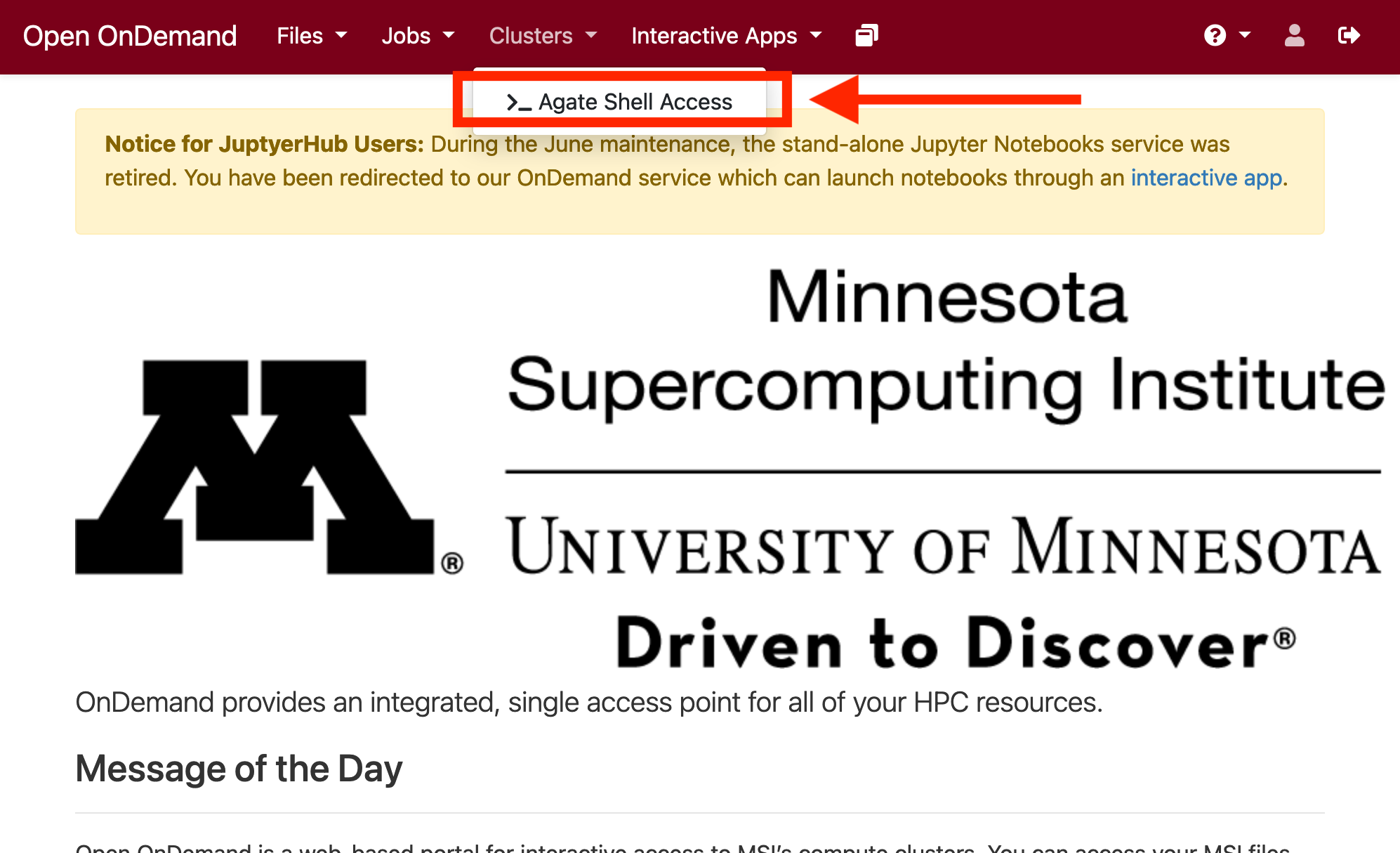
In this tutorial, we will use the MSI Open OnDemand (OOD) service to access a command line interface. Open a web browser and navigate to https://ood.msi.umn.edu/. Log in with your UMN user name and password. You will see a screen like the one shown below:

Click on the Clusters button. A drop-down menu will fold out. Click on
Agate Shell Access:
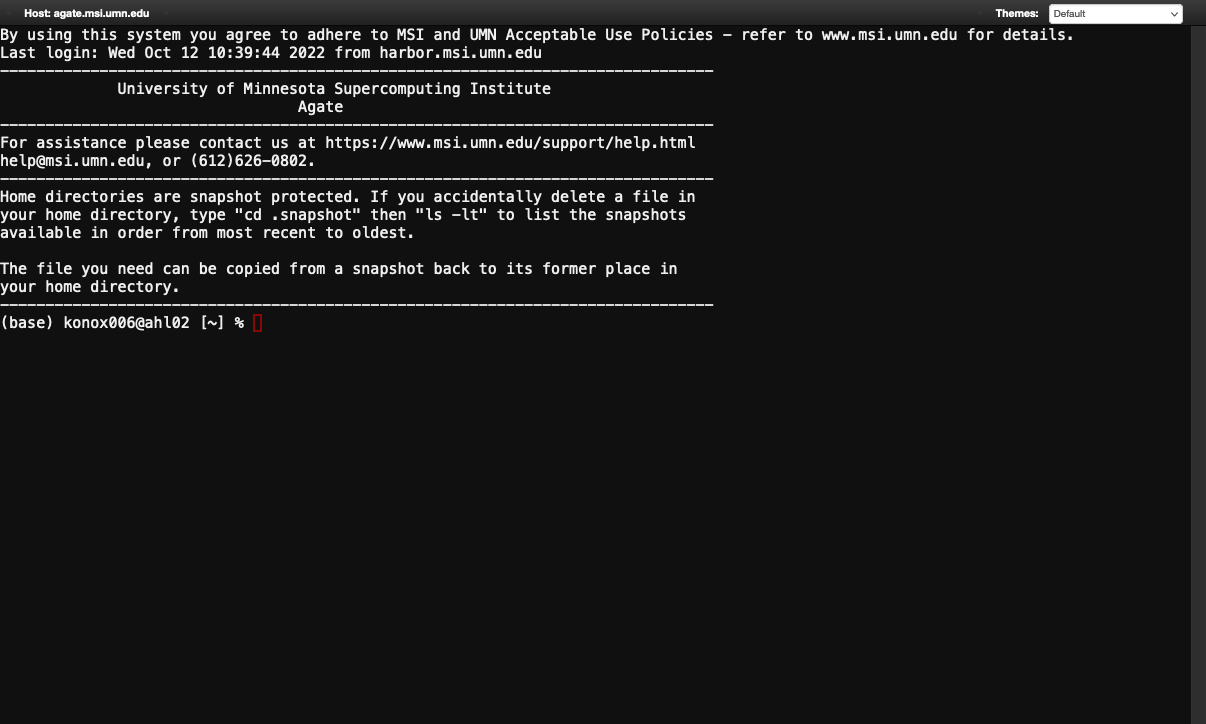
A new tab will open with a command line prompt. You can change the appearance
with the Theme: drop-down menu.
The portion of the prompt to the left of and including the percent symbol (%)
is called the “prompt.” The block is called the “cursor.” When you type
commands into the command line, the symbols will appear to the left of the
cursor:
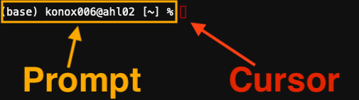
Note that my prompt may look different from yours! The function is identical, regardless of appearance.
Note that you cannot use the mouse to move the cursor around in the terminal area! You must use the arrow keys to move the cursor to edit the command you are currently typing. We will cover this later when we start entering actual commands!
Before we start to write and enter commands at the command prompt, though, we will go over directory and file structure on MSI systems.
Other ways to access a command line on MSI systems
-
Web Browser (any platform)
Navigate to https://notebooks.msi.umn.edu/. Choose the MSI group in which you would like to run the command line. Click the blue
Start My Serverbutton. SelectBasic Interactivefrom the list of job profiles, then click the orangeStartbutton. The page will display the job submission and queue progress. When the job launches, you will see a grid of app launchers. Scroll to the bottom of the list and click on theTerminalicon (under the “Other” section). -
Mac OS X Workstation:
Hold the
commandandshiftkeys and press theakey to open the Applications folder. Open the “Utilities” folder, and double-click on “Terminal.” You must first click on a Finder window or the desktop window before the keyboard shortcut will work. -
Linux Workstations in Walter Computer Lab:
Click the menu icon on the top left of the screen, then hover over “Applications,” then “System Tools,” and then click on “Terminal.”
-
Personal Linux Workstation:
Run your preferred terminal emulator application. Unfortunately, the name and location of the application varies by distribution and version. The most common distributions of Linux will have a similar layout to the SDVL workstations.
-
Windows Workstation:
You will need to install additional software to use a command line interface. The software that MSI recommends is called PuTTY, and is available for download at https://www.chiark.greenend.org.uk/~sgtatham/putty/latest.html. MSI maintains a setup guide for PuTTY here: https://www.msi.umn.edu/support/faq/how-do-i-configure-putty-connect-msi-unix-systems.
For Windows 10 machines, the Bash subsystem (https://docs.microsoft.com/en-us/windows/wsl/install-win10) should allow you to run a terminal emulator and connect to MSI systems without the PuTTY application. Similar to the Linux laptop case, the way to launch a terminal emulator application will depend on which distribution you choose to install.
For PuTTY users, the process for connecting to MSI servers is somewhat different than for the other methods. Please follow the instructions in the MSI PuTTY guide (https://www.msi.umn.edu/support/faq/how-do-i-configure-putty-connect-msi-unix-systems) to connect.
For the Mac OS and Linux methods, type
ssh YOUR_ID_HERE@agate.msi.umn.edu then press Enter. Enter your password
if you are asked for it. Note that you will not be able to see any text entry
as you type your password; this is normal. After you finish entering your
password, press Enter again. You will be prompted to authenticate the login
attempt with DUO.
2.3: Directories and Files
Understanding files and directories is one of the key pieces of using a UNIX-like system (which includes MSI systems). One of the defining characteristics of UNIX-like systems is that “everything is a file.” This means that everything that the computer can interact with, including input and output devices, is represented as a file on the filesystem. Keyboards, mice, monitors, hard disks, executable programs, data - these are all represented as files. You generally will not have to interact with the files that represent the computer hardware, but you will have to navigate the filesystem to find the programs that you want to use to analyze your data and point these programs at your data set.
The image that is often used to illustrate the concept of the directory and file structure is a tree. In this metaphor, a directory is a branch and a file is a leaf. Branches can contain multiple other branches and leaves. On Windows and Mac OS (and other common desktop operating systems), directories are often called “folders,” so you can think of these as interchangeable terms.
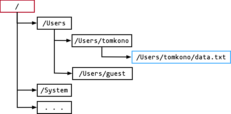
In the tree cartoon above, boxes represent directories or files, and indentation
represents nesting. The text inside the boxes represents the names. The red
box (around /) represents the root of the filesystem, and the blue box
(around /Users/tomkono/data.txt) represents a file. The boxes in black
are directories.
Just like in evolutionary biology, a tree structure does not really capture the relatedness of directories and files. Some special types of files are actually links to paths in the filesystem that are very divergent from where the locations of the link files are, like reticulations in a phylogenetic tree. There is optional material later in this tutorial that will show you how to make links. These are very useful for making a dataset easy to find without having to actually copy the raw data.
Notice the slashes (/) between parts of the names - these delimit the actual
directories that make up the full path to the file. In the case of
/Users/tomkono/data.txt, you can read the name and know that the file called
data.txt is located under the root (/), then the Users directory, then
the tomkono directory. In UNIX terminology, this is known as the path to
the file. More specifically, it is known as the absolute path because it
starts at the root of the filesystem. This is the way I prefer to specify paths
to files because there is no ambiguity as to where the file is located.
A path that does not start at the root is known as a relative path. To really show the difference between absolute paths and relative paths, we will have to run a few commands, so we will start to do that now.
When typing file paths, be sure to include the root slash at the beginning. A
path of Users/tomkono/data.txt means something very different from the path
/Users/tomkono/data.txt.
2.4: Basic Commands and Exercises
2.4.1: The Structure of a Command
A UNIX or Linux command consists of a program, options, and arguments. The
program is what actually does something to a file. The options modify the
behavior of the program. The arguments are the files on which the program
operates. The parts of a command are separated by spaces, so be sure to
include those as you follow along with the examples in the next section. A
command is completed with the Enter key.
Sometimes, as you will see in the next section, the arguments are not required. In cases where the argument is not required, a default value will be substituted in to the command. You should double-check that the program will work as intended with the default values before you run them.
Note that mouse support is very limited in most terminal programs. You can
highlight and copy text with the mouse, but you must use the arrow keys to
move the cursor around. The left and right arrow keys will move you
backward and forward within the current command, and the up and down arrow
keys will move you earlier and later in the command history.
Also note that all parts of a command are case sensitive. That means that
capitalization matters. A is different from a.
2.4.2: Running Commands
The first command we will run is one that will change directories. This is how
we navigate the filesystem. The command is called cd for “change directory.”
Type cd then a space, then the path to where you would like to go. We will
go to the /commmon/tutorials/bioinformatics/ directory. Press Enter when you have finished
typing the command:
cd /common/tutorials/bioinformatics/

Notice how your prompt updates to let you know that you are now in a different
directory than when you started. This is a quick way to check where you are
currently working. You can verify this with the pwd command. Type pwd then
Enter to print the working directory:
pwd

Next, we will list the contents of the current working directory. We use the
ls command to do this. Type ls then Enter:
ls

There are multiple items under /commmon/tutorials/bioinformatics/. The blue coloring indicates
that they are directories. Let’s cd into the pathway_analysis
directory now and list contents again:
cd pathway_analysis
ls
cd Test_Data
ls

Note that we did not specify a leading slash (/) on this command. This is
because we want to go into a directory that is relative to our current
working directory. We will come back to this directory later. It has the test
data set that you will use for the next part of the tutorial. For now, we will
make a directory to hold the output files from the pathway enrichment analysis.
We will navigate to global scratch. This is a special part of the MSI
filesystem where you can write temporary data. We will use it to hold the
output files from the pathway analysis that will be run later in this tutorial.
The global scratch directory is called /scratch.global (note the leading
slash; this is an absolute path!):
cd /scratch.global/

Next, we will make a new directory with the mkdir command. Because global
scratch is a public area, it can be difficult to keep track of which data are
yours. To help organize it, we will make a directory that has your name on it
so you can always find your files. Type mkdir, then a space, then your
UMN internet ID, then Enter:
mkdir mmacchie_tut

Again, we do not have to specify the full path to the new directory because we
are making it relative to the working directory, which is /scratch.global.
Let’s cd into the directory that we just made:
cd mmacchie_tut

Next, we will copy a file into our current directory. We use the cp command
to do this. cp takes two arguments, a source and a destination. For this
exercise, the source will be a long path name:
/common/tutorials/bioinformatics/pathway_analysis/Test_Data/Drosophila_melanogaster_edgeR_DEG_table_full.txt
and the destination will be the current working directory. This is
shorthanded by a dot (.) in the command:
cp /common/tutorials/bioinformatics/pathway_analysis/Test_Data/Drosophila_melanogaster_edgeR_DEG_table_full.txt .

Note that the line wrapping in the terminal has no function on the command. It just might make it a bit more difficult to read, unfortunately. Once you run this command, you can list the directory contents to verify that you have successfully copied the file:
ls

These are mostly the commands you need to know to follow along with this tutorial. There are additional resources below, but they are not required for you to use our script for pathway analysis.
To recap:
cd: change directorypwd: print working directoryls: list directory contentsmkdir: make new directorycp: copy file
From this point on, commands will only be written in monospace typeface and
the prompt will not be included. For the ease of copying and pasting commands,
we will not include screenshots.
2.5: Other Useful Commands
There are many more commands that exist on a UNIX or Linux system. There are
several dozen that I know very well because I use them on a daily basis. One of
the most useful commands is man, which brings up a manual page for a certain
command. Manual pages list all of the available options for a given program. If
you want to know all of the ways that the behavior of a program can be modified,
check the manual!
More about reading manual pages, with example
For instance, if you wanted to view a manual page for the mkdir
command, you would type man mkdir:
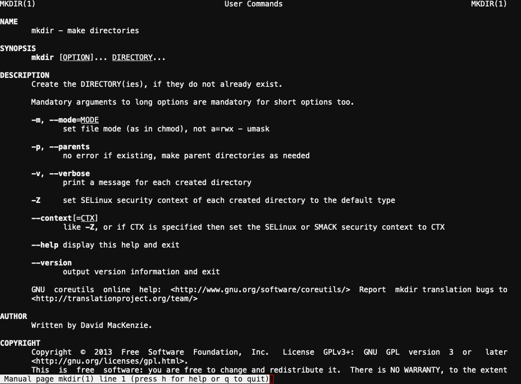
Use the arrow keys to scroll up and down in the manual page. Press the q key
to quit out of a manual page viewer.
Now that you know the command to view the manual, you can check the manual to see how to use these next commands! These are commands I use on a near-daily basis to slice up data files to prepare them for various bioinformatic workflows or take a peek at the contents of a file without trying to load the entire file into memory.
head: Print the first lines of a file to the terminaltail: Print the last lines of a file to the terminalgrep: Search for text within a filecut: “Cut” out and return certain columns from a fileless: View the contents of a file in the same way you view a manual pageln: Make links to other files and directoriesfind: Find files and directories that match a certain name patterncat: Print one or more files directly to the terminalrm: Delete a file. Once it’s gone, it’s gone! No recycle bin or trash*wget: Download remote files (from websites) to disk
*: MSI home directories (/home/PI_group/) have snapshot backups available in
the .snapshot directory under the main directory. You can recover files from
these directories so long as the file at least one day old. The snapshots
go back on month from the from the current day. Global scratch is
not backed up by snapshots, so when you delete data from there, it is gone
for good.
A Note on ln
Linking a file is a very useful way to make it available in other directories without having to copy it. A link looks like a regular file, but is actually a reference or alias to another location on disk. We recommend using symbolic links rather than hard links. Without getting too technical, a symbolic link (“symlink” for short) behaves as a separate file from the data to which it points. A hard link references the exact same data, so if you delete a hard link, the source data is also deleted.
Examples of making symbolic links
To make a symlink, use the -s option to ln. The syntax is as follows:
ln -s /long/path/that/is/annoying/to/type/to/data.txt /easy/path/to/data.txt
This will make a file at /easy/path/to/data.txt that will reference the actual
file at /long/path/that/is/annoying/to/type/data.txt. It will happen
very quickly because no actual data copying is involved, and the source data
is preserved in terms of access time and modification time. You can also link
to directories:
ln -s /long/path/to/UMGC/data_delivery /easy/path/to/data
This will make a file that looks like a directory at /easy/path/to/data that
references /long/path/to/UMGC/data_delivery. Again, the original directory and
file attributes are preserved.
You can safely remove symlinks with rm while leaving the source data intact.
I make a big deal out of preserving access/modification time and filenames, but this is because it is a very important issue. It is common for researchers to collect datasets over a long period of time and use the time of file creation to keep track of when a dataset was collected or generated.
But, note that a symbolic link will be broken if the source data are deleted or moved! Also, making a symbolic link is not sufficient for purposes like backing up or archiving data!
There are many versions of UNIX out there, and some of these commands have different default behaviors and different options, depending on which version you are using. For example, Mac OS X is technically a UNIX, and has all the standard commands listed above, but they behave differently from the tools installed on MSI systems, which is GNU/Linux. If you are unsure of what a command will do, check the manual page!
Part 3: Running and Interpreting Pathway Analyses
This section will be dedicated to demonstrating how to run a pathway analysis using a script that was developed by MSI-RI. We will also cover how to read the outputs of the script and interpret the results of a pathway analysis.
Please note that the MSI script uses functions, visualization routines, and
terminology from the clusterProfiler R package (https://www.bioconductor.org/packages/clusterProfiler).
3.1: Connect to an Interactive Node
Before we run any pathway analyses, we must connect to an interactive or compute node to request more computational resources.
Navigate back to the terminal we opened before through https://ood.msi.umn.edu/. In the commandline, type:
srun -N 1 -n 1 -c 1 --mem 32gb -t 2:00:00 -p interactive --pty bash
The command above will request 1 node (-N 1), 1 task (-n 1), 1 cpu (-c 1), with 32 Gb of memory (–mem 32gb), for 2 hours (-t 2:00:00), from the interactive partition (-p interactive).
These resources are appropriate for the tutorial dataset, which contains data from 13,632 genes in Drosophila melanogaster. This is typical for the size of a Eukaryotic bulk RNAseq experiment, but if you find that you are running into memory errors or getting segmentation fault errors, try increasing the value for “Memory per Node.”
3.2: Load the Pathway Analysis Module
We will load the pathway analysis software module.
Enter or paste the following command into the terminal:
module load clusterprofiler_wrapper/2.1
Test that the module was successfully loaded by running the pathway analysis script with the “help” option:
run_clusterProfiler.R -h
If you see a long message that gives you a list of options for customizing the pathway analysis, then the script has been successfully loaded and it is ready to run pathway analysis with a list of genes.
3.3: Run Pathway Analysis Script
These next sections will guide you through running the pathway analysis script from the command line and inspecting the outputs.
3.3.1: Run ORA with Default Parameters
We will first run a “simple” ORA using the gene expression results from a Drosophila melanogaster experiment. Navigate back to your global scratch directory in the terminal emulator:
cd /scratch.global/YOUR_ID_HERE
where YOUR_ID_HERE is your UMN internet ID. Run the script with the command
below:
run_clusterProfiler.R \
    Drosophila_melanogaster_edgeR_DEG_table_full.txt \
    Drosophila_melanogaster \
    SYMBOL
The first argument is the DEG table that you would like to use for testing
pathway enrichment. The second argument is the genus and species of the study
system, and the third argument is the type of gene identifier that is used in
the DEG table. In this case, the organism is Drosophila_melanogaster and we
are using gene symbols.
This will take a minute or two to complete. While the script runs, text will be written to the terminal that shows the progress of the analysis.
To view the outputs, we will open a new tab in a web browser and navigate to the MSI OpenOnDemend webpage: https://ood.msi.umn.edu/
Click the “Files” drop down menu, and click on the folder that you created in /scratch.global/.
The results from the pathway analysis script are stored in the directory
called clusterProfiler_results. Double-click on the icon for this directory
to open it and browse its contents.
The PDF figures display the plots that were described in Part 1 of this
tutorial (the Google Slides presentation). These are dotplot files,
cnetplot files, and emapplot files.
The Parameter_settings.txt file describes the FDR, log2(fold change), and
gene number thresholds that were used for the pathway analysis. It also lists
the gene sets and gene ontology terms that were tested for enrichment. The
settings recorded in this file are essential to describe and reproduce the
results of the pathway analysis.
The text files whose names start with Table_ give the tabular results of the
pathway analysis, also described in Part 1 of this tutorial. If you would like
to make custom visualizations or plot only subsets of the pathway analysis
results, then you can use the information stored in these files.
The sessionInfo.txt file gives the names and versions of the R packages that
were used during the pathway analysis. The information in this file is required
for describing the software environment in which the analysis was conducted.
3.3.2: Run ORA With GSEA
Next, we will run an ORA and also include a gene set enrichment analysis (GSEA). Enter the following command into your terminal emulator window:
run_clusterProfiler.R \
    Drosophila_melanogaster_edgeR_DEG_table_full.txt \
    Drosophila_melanogaster \
    SYMBOL \
    --gsea=TRUE \
    -d Dmel_results_GSEA
Note that we added options --gsea=TRUE to enable GSEA and
-d Dmel_results_GSEA to make a new directory for the results. This will take
slightly longer to run than the previous command because it is running
additional tests and generating additional visualizations.
You should see a new directory has been created in your global scratch directory
called Dmel_results_GSEA. This directory will have all of the same outputs as
the original clusterProfiler_results directory from the previous section, but
with additional files. The msigdb_gsea directory will have the results of
GSEA against the Molecular Signatures Database (MSigDB) pathway set, and the
suppl_files directory will have the ranked list that was used for the GSEA.
Within the msigdb_gsea directory, there are directories corresponding to each
collection that was tested. In this example, there is only one directory for
h, corresponding to the “Hallmark Gene Sets” collection from MSigDB. The h
directory contains PDF figures of the enrichment plots for each gene set that
is significantly enriched in your gene list.
3.3.3: Run ORA with GSEA and Multiple Gene Sets
Next, we will run the pathway analysis script again, but include additional gene sets from MSigDB to test. Enter the following command into your terminal emulator:
run_clusterProfiler.R \
    Drosophila_melanogaster_edgeR_DEG_table_full.txt \
    Drosophila_melanogaster \
    SYMBOL \
    --gsea=TRUE \
    -d Dmel_results_GSEA \
    --msigdbs h,c2_cp_reactome,c5_go_bp,c2_cp_kegg
See that we added the option --msigdbs h,c2_cp_reactome,c5_go_bp,c2_cp_kegg
to explicitly define the MSigDB collections that we would like to use. In this
case, we are using the Hallmark gene sets (h), the Reactome gene sets
(c2_cp_reactome), the GO Biological Process gene sets (c5_go_bp), and the
KEGG gene sets (c2_cp_kegg).
Navigate to the output directory to view the outputs of the GSEA run against the additional gene sets.
3.3.4: Customizing the Pathway Analysis
Recall that when you ran the pathway analysis script with the help option
(-h), you were shown a list of options for adjusting the behavior of the
pathway analysis. Simply add these to the command to change the parameters of
the pathway analysis. For example, to change the FDR threshold for DEG
inclusion the default 0.05 to a more lenient value of 0.1 for the ORA, you
can write a command like this:
run_clusterProfiler.R \
    Drosophila_melanogaster_edgeR_DEG_table_full.txt \
    Drosophila_melanogaster \
    SYMBOL \
    -p 0.1
If you wanted to additionally change the maximum number of genes that would be
included in the ORA from the default 200 to 400, you could write:
run_clusterProfiler.R \
    Drosophila_melanogaster_edgeR_DEG_table_full.txt \
    Drosophila_melanogaster \
    SYMBOL \
    -p 0.1 \
    -g 400
These options (-p and -g) do not affect the genes that get included in GSEA,
which uses all genes in the DEG file. We recommend running GSEA with every gene
that was tested for differential expression because the signal from GSEA comes
from the expression responses of all genes, significantly DE or not.
Because the nature of a pathway analysis is exploratory, it may be worthwhile to run the analyses with various filtering criteria to see what pathways are enriched in your DEG list. If the pathways change drastically from run to run, then it suggests that the biological signal in your results is not very strong.
Do keep in mind the suggestions for gene number to be included in ORA, however. If you include too many genes, then your results will be difficult to interpret. This is because there will likely be a lot of noise in the gene set. Similarly, if you include too few genes, the results will be difficult to interpret because very small hits will look significantly enriched. For example, if your DEG list includes 10 genes, one gene occurring in a pathway may make the pathway look significantly enriched because 10% of your DEG list occurs in it. However, just one gene being significantly DE is likely not a biologically relevant enrichment.
There is unfortunately no rule for the “right number” of genes to include, but between 150 and 500 is a “good” number for ORA.
For a full description of the options available to the pathway analysis script, please see https://github.umn.edu/MSI-RIS/clusterProfiler_wrapper.
3.3.5: Analyzing Data from Other Species
The tutorial dataset was derived from Drosophila melanogaster, but the
clusterProfiler_wrapper script supports multiple species. At the time of
writing, a total of 12 species are supported, summarized in the table below.
If a species does not have an entry in a given column (e.g., Bos taurus for
Reactome), then that species does not have data in the database. At present,
all 12 species have support from the base Bioconductor annotation package and
KEGG. Only cattle (Bos taurus), chicken (Gallus gallus), and swine
(Sus scrofa) do not have Reactome support.
| Species | Bioconductor Annotationdb | KEGG Code | Reactome Code |
|---|---|---|---|
| Bos taurus | org.Bt.eg.db |
bta |
|
| Caenorhabditis elegans | org.Ce.eg.db |
cel |
celegans |
| Canis lupus familiaris | org.Cf.eg.db |
cfa |
canine |
| Danio rerio | org.Dr.eg.db |
dre |
zebrafish |
| Drosophila melanogaster | org.Dm.eg.db |
dme |
fly |
| Gallus gallus | org.Gg.eg.db |
gga |
|
| Homo sapiens | org.Hs.eg.db |
hsa |
human |
| Mus musculus | org.Mm.eg.db |
mmu |
mouse |
| Rattus norvegicus | org.Rn.eg.db |
rno |
rat |
| Saccharomyces cerevisiae | org.Sc.eg.db |
sce |
yeast |
| Sus scrofa | org.Ss.eg.db |
ssc |
To target the analysis against a given species, use the name in the first
column, with spaces replaced by underscores (_). Note that the names are
case-sensitive. For example, to analyze a dataset from mouse, you might
use a command like so:
run_clusterProfiler.R \
    Full_DEG_Table.txt \
    Mus_musculus \
    SYMBOL \
3.4: Transferring Results to Local Workstation
To transfer the results from MSI systems to your local workstation, open a new web browser tab on your workstation and navigate back to https://ood.msi.umn.edu/. Click on the “Files” menu, then click on “Home Directory” to open the Open OnDemand file browser.
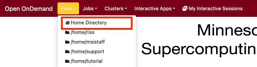
Click the “Change directory” button and enter the path to the scratch directory where we have been doing our analyses. Click the “OK” button. The display will update to show you the contents of the scratch directory. You can click on the names of the directories to navigate through the results of your pathway analysis.
To download an individual file, click on the checkbox next to its name to select it, then click the “Download” button to save the file to your workstation. You can also do this to download entire directories. When you download a directory, the contents will be served as a zip file.
3.5: Customizing clusterprofiler Pathway Figures
If ORA figures (dotplot, emapplot, cnetplot) are not formatted to your preference, the R .rds files produced by the clusterprofiler_wrapper script (boxed in red in the screenshot below) can be loaded into R, and figures can be re-made using the clusterprofiler R package’s visualization functions. We will cover how to generate the dotplot (dotplot()), emmaplot (emappplot()), and cnetplot (cnetplot()) figures using the functions.

Here are steps to load R 4.3 through the clusterProfiler_wrapper module and generate plots using the .rds files.
module load clusterprofiler_wrapper/2.1
Then, we will load the R version from the clusterprofiler_wrapper software module we just loaded, by typing:
R
Now that we are in R, we can load the clusterprofiler R package, and one of the GO, KEGG, or REACTOME .rds files:
# Load the required R packages
library(clusterProfiler)
library(enrichplot) # Needed for emapplot

# Load the GO term ORA Results object
results_object <- readRDS("/path/to/GO_enrichment_results.rds")
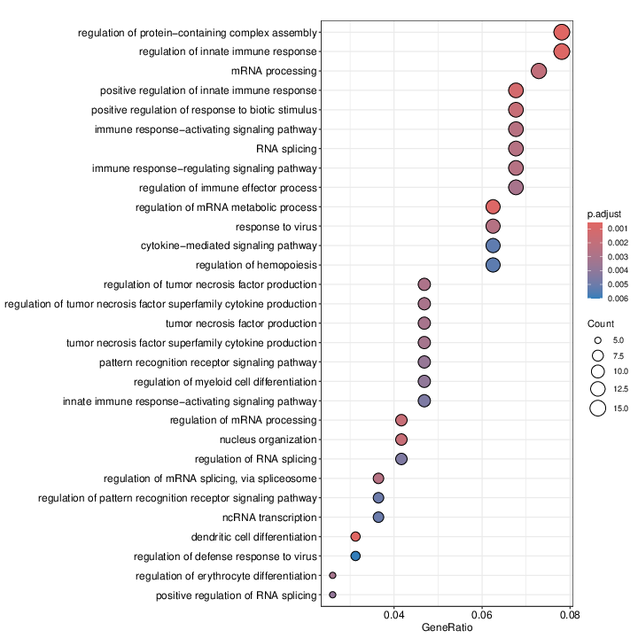
Once the file is loaded as results_object in this example, we can run the dotplot() function adjusting the parameters to our preference, and save the plot as a PDF image. The height and width of the image can be adjusted those the image_height and image_width variables.
All dotplot parameters can be viewed here: https://rdrr.io/bioc/enrichplot/man/dotplot.html
Dotplot
#########################################
# Plot a dotplot as a PDF figure
########################################

# Set the image height and width (adjust this)
image_height=10
image_width=10

pdf("Dotplot_GO_ORA_custom.pdf",h=image_height,w=image_width)
     dotplot(
       results_object,
       x = "GeneRatio", # variable to plot on the x-axis
       color = "p.adjust", # Color of the dots
       showCategory = 30, # number of ORA pathway terms
       size = NULL,
       split = NULL,
       font.size = 12,
       title = "", # Set your title here
       orderBy = "x", # Order the values on the x-axis
       label_format = 80) # The number of characters (of a pathway term label) that will display on one line. Increase if you don't like the label displaying across multiple lines.
dev.off()
Emapplot
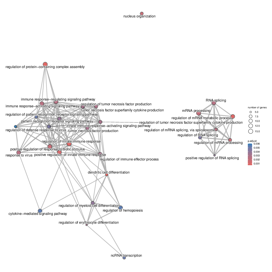
Now, let’s generate an emapplot with the following R code. All emapplot parameters can be viewed here: https://rdrr.io/bioc/enrichplot/man/emapplot.html
#########################################
# Plot an emapplot as a PDF figure
########################################

# Set the image height and width (adjust this)
image_height=15
image_width=15

# Add similiarity matrix to the termsim slot of the results object [required for emmaplot to work]
results_object <- pairwise_termsim(results_object)


# Save emapplot to PDF
pdf("Emapplot_GO_ORA_custom.pdf",h=image_height,w=image_width)
     emapplot(results_object,
        showCategory = 30)
dev.off()
Cnetplot
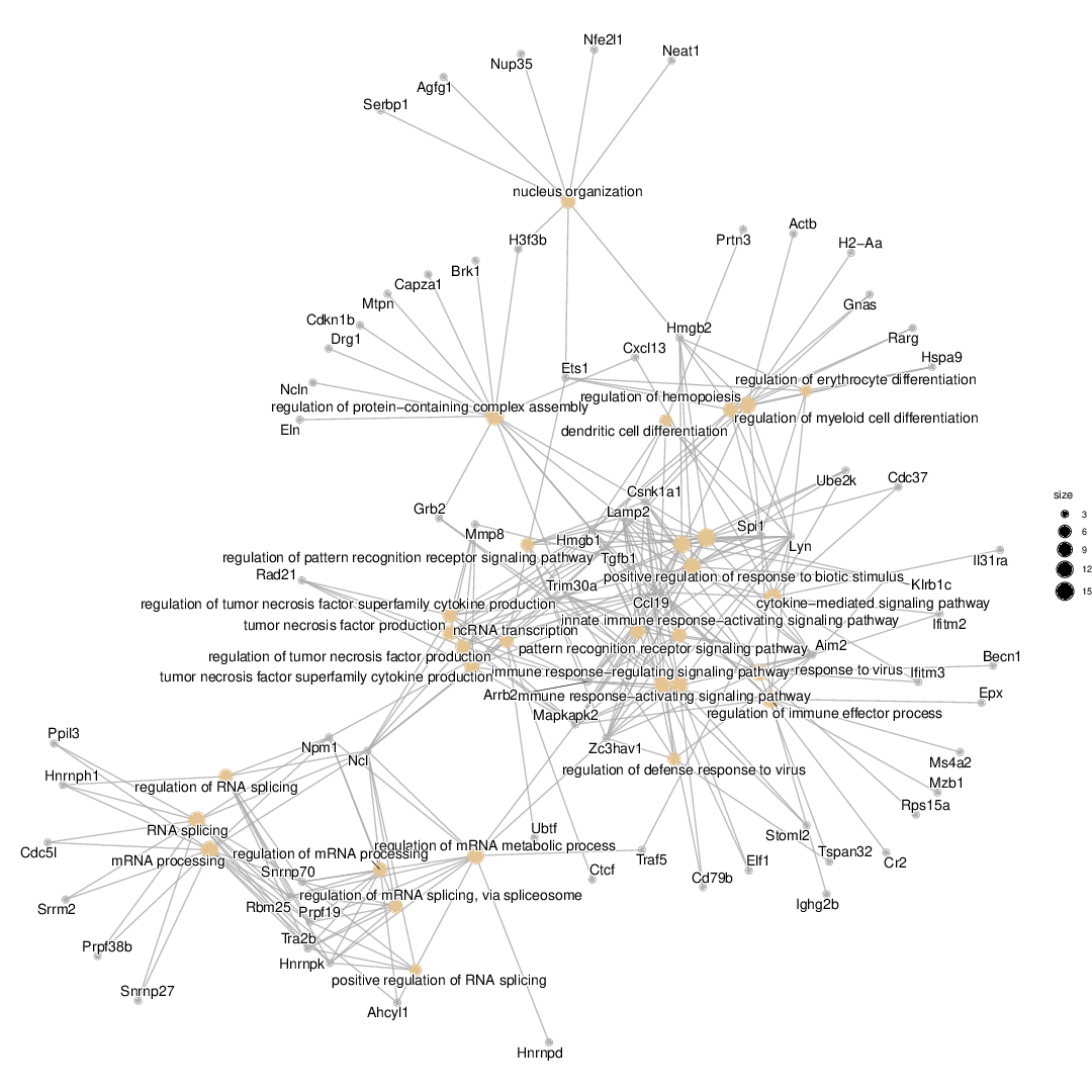
Now, let’s generate an cnetplot of the enrichment results with the following R code. Note: we do not have fold change information within these enrichment result objects, so the genes will not be color-coded by their fold changes on this plot. The fold change data from the DEG table can be included in the cnetplot() with the foldChange parameter.
All emapplot parameters can be viewed here: https://rdrr.io/bioc/enrichplot/man/cnetplot.html
#########################################
# Plot an cnetplot as a PDF figure
########################################

# Set the image height and width (adjust this)
image_height=15
image_width=15

# Add similiarity matrix to the termsim slot of the results object [required for emmaplot to work]
results_object <- pairwise_termsim(results_object)


# Save emapplot to PDF
pdf("Cnetplot_GO_ORA_custom.pdf",h=image_height,w=image_width)
     cnetplot(results_object,
        showCategory = 30,
        foldChange = NULL) # Optional - Add vector of log2 fold change values here. Names on the values in the vector should be gene IDs.
dev.off()
Part 4: Feedback
This tutorial was prepared by the RI group at MSI. If you have suggestions for
improvement or topics that you would like to see covered, please send an
email to help [at] msi.umn.edu and include “Pathway Analysis Tutorial
Feedback” in the email subject line.