Please see http://z.umn.edu/ris-rnaseq/ for the latest version of this tutorial document!
RNASeq Analysis With CHURP
Last Updated: 2026-05-27
Last Delivered: 2026-04-07
Check out the recording of this tutorial and other MSI tutorials on our YouTube channel: https://www.youtube.com/@UofMMSI/videos
Expand all details (Useful for printing!)
Collapse all details
Part 0: Introduction
This tutorial will cover the basic use of the CHURP workflow for bulk RNAseq data analysis. The tools are used via the Linux command line. We cover important aspects of data QC and considerations to take when interpreting RNAseq results.
CHURP is published here: https://doi.org/10.1145/3332186.3333156 and is fully supported by RI:Bioinformatics.
Outline
- Overview of steps in RNASeq
- Interactive tutorial using CHURP pipeline on MSI to conduct RNASeq analysis
- Examination of output / results
- Next Steps
Part 0.1: Goals
By the end of this tutorial you should be able to:
- Understand the inputs, outputs, and main steps in Bulk RNASeq
- Use the CHURP workflow to generate relative gene expression data from RNAseq fastqs
- Assess the quality of your libraries with post-lab metrics
- Identify differentially-expressed genes among experimental groups using the automated DEG testing routines
Part 0.2: Scope of the Tutorial
What this tutorial covers
- Overview of most common steps in a bulk RNASeq workflow
- Usage of MSI’s CHURP RNASeq pipeline on the agate supercomputing cluster
- Overview of results interpretation
- Description of common downstream steps
What this tutorial DOESN’T cover
- a detailed guide to the command line
- a detailed guide to running jobs on MSI’s clusters
- the specific parameters used by each internal program in the CHURP pipeline
- single cell, small RNA, differential splicing, etc.
For discussion of project-specific settings and next steps, see the supplementary sections at the end of this document.
Part 0.3: Prerequisites
- Ability to access MSI’s agate cluster on the command line:
https://www.msi.umn.edu/content/connecting-hpc-resources
- Command line navigation. While we will go over the commands needed for submitting CHURP, a more detailed linux command line guide is here:
https://pages.github.umn.edu/dunn0404/intro-to-linux/
or here:
http://hpcc.ucr.edu/manuals_linux-basics_cmdline-basics.html
- Biology behing RNASeq (central dogma, molecular bio, etc.)
Part 0.4: Formatting
Throughout this tutorial, there will be formatting cues to highlight various pieces of information.
This is just background information. There are no tutorial-related tasks in these boxes. Links to supporting material and further explanations of points we raise in the tutorial will appear like this.
This is a warning. Common pitfalls, cautionary information, and important points to consider will appear like this.
This is code, or a literal value that you must enter or select to run a part of the tutorial
These boxes contain detailed information. Click on them to expand them
When you click on these boxes, you will get a detailed view into a technical topic. The information in these boxes may be useful for advanced work beyond the scope of the tutorial We encourage you to read these, but they are not essential to completing the tutorial!
Part 1: Bulk RNASeq steps
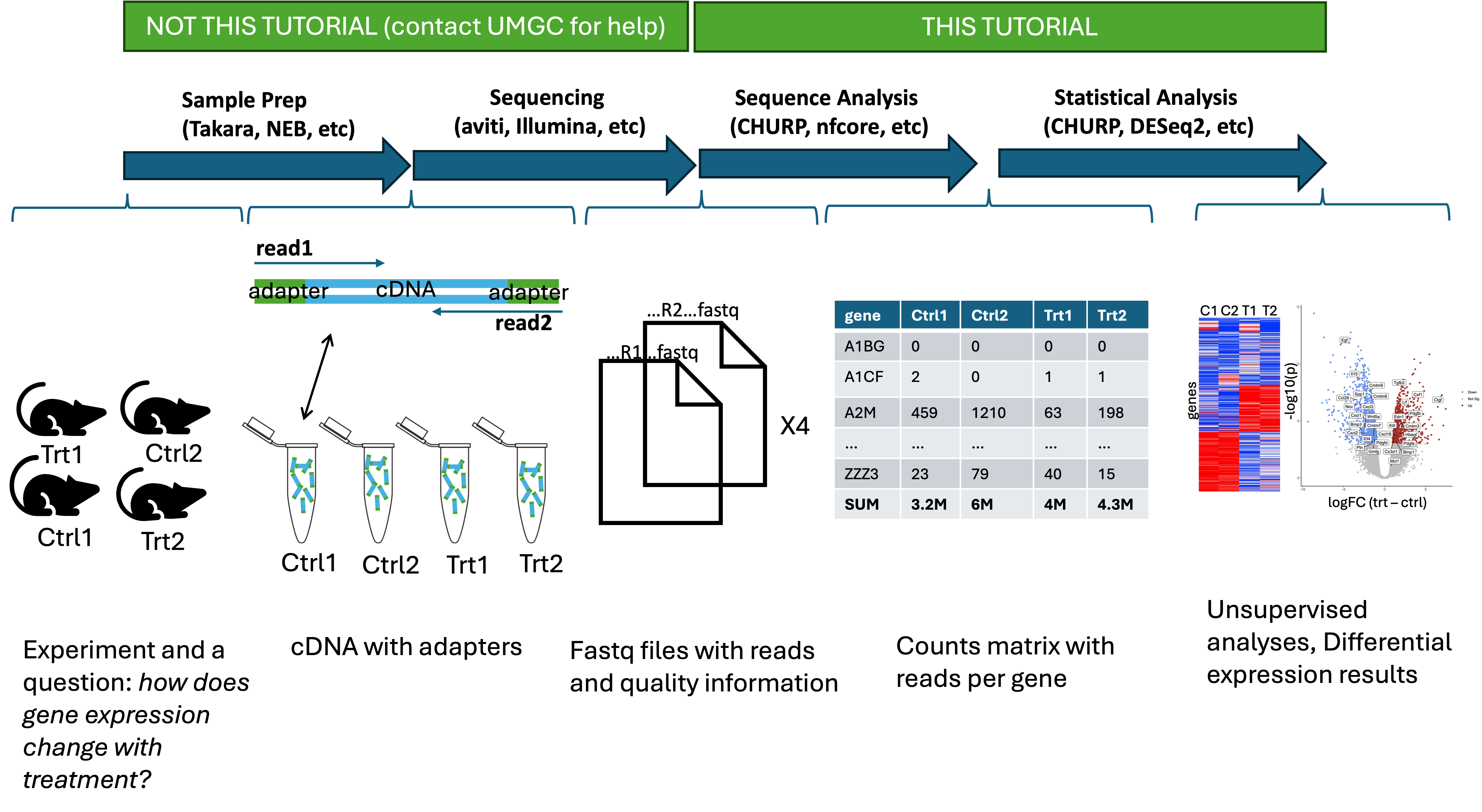
Main steps of bulk RNASeq
- Do a controlled experiment and prepare RNA for sequencing
- Sequence the cDNA and produce fastq files
- Process the sequence files (fastqs) into a counts matrix
- Statistically analyze the counts matrix
Details of the RNASeq study files we use in this tutorial:
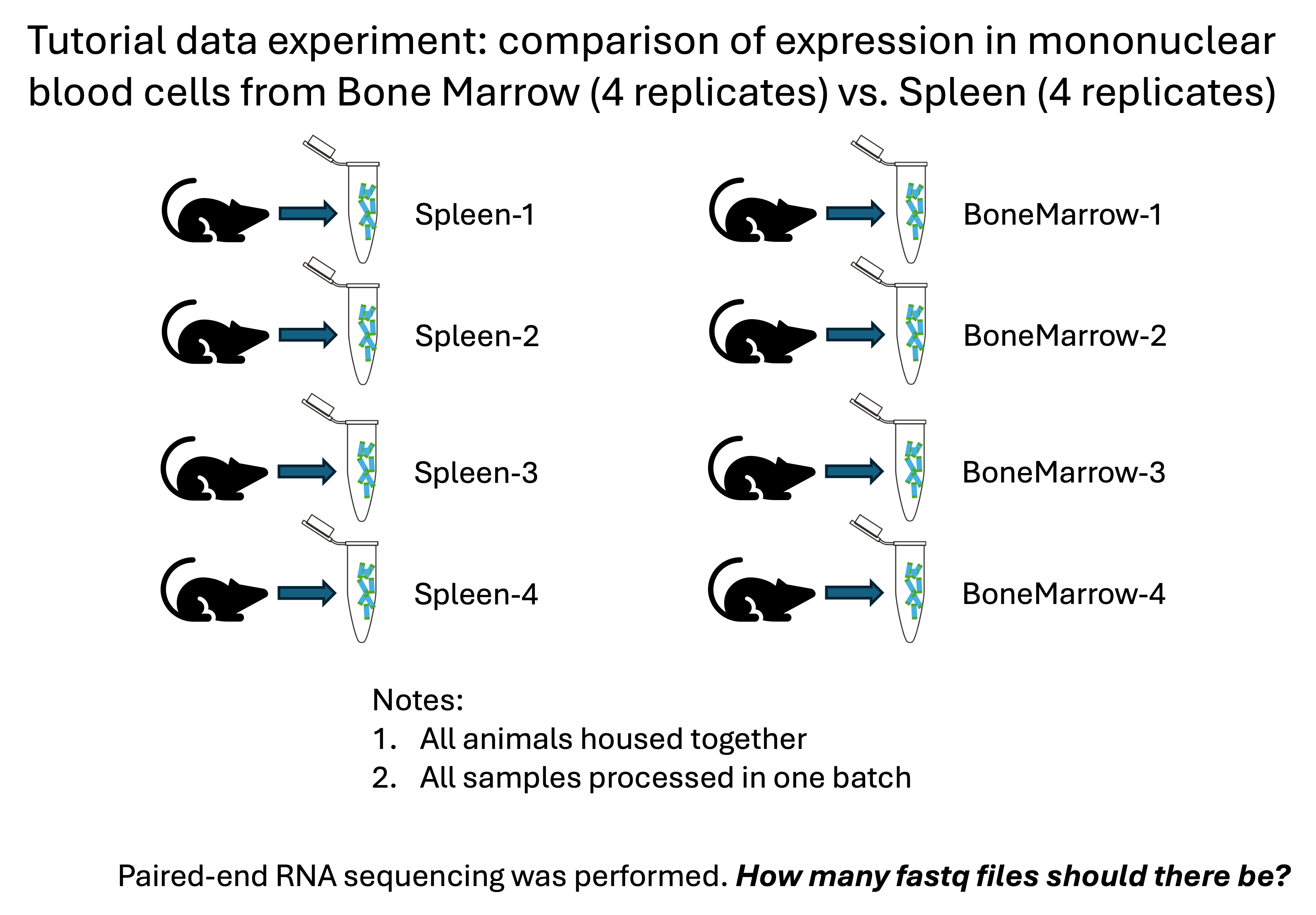
The dataset we will use for this live tutorial are from a mouse RNASeq experiment.
Part 2: Using and Accessing the Command Line on MSI
Accessing MSI systems requires that you either be connecting through the UMN
network (eduroam or Ethernet in a UMN building) or connected to the UMN
VPN. Please see https://it.umn.edu/services-technologies/virtual-private-network-vpn
for information on connecting to the UMN VPN.
You will also be required to have DUO multi-factor authentication set up. Please see https://it.umn.edu/services-technologies/self-help-guides/duo-set-use-duo-security for information about enrolling your device in DUO.
Other ways to access a command line on MSI systems:
-
Mac OS X Workstation:
Hold the
commandandshiftkeys and press theakey to open the Applications folder. Open the “Utilities” folder, and double-click on “Terminal.” You must first click on a Finder window or the desktop window before the keyboard shortcut will work. -
Personal Linux Workstation:
Run your preferred terminal emulator application. Unfortunately, the name and location of the application varies by distribution and version. The most common distributions of Linux will have a similar layout to the SDVL workstations.
-
Windows Workstation:
You will need to install additional software to use a command line interface. The software that MSI recommends is called PuTTY, and is available for download at https://www.chiark.greenend.org.uk/~sgtatham/putty/latest.html. MSI maintains a setup guide for PuTTY here: https://www.msi.umn.edu/support/faq/how-do-i-configure-putty-connect-msi-unix-systems.
For Windows 10 machines, the Bash subsystem (https://docs.microsoft.com/en-us/windows/wsl/install-win10) should allow you to run a terminal emulator and connect to MSI systems without the PuTTY application. Similar to the Linux laptop case, the way to launch a terminal emulator application will depend on which distribution you choose to install.
For PuTTY users, the process for connecting to MSI servers is somewhat different than for the other methods. Please follow the instructions in the MSI PuTTY guide (https://www.msi.umn.edu/support/faq/how-do-i-configure-putty-connect-msi-unix-systems) to connect.
For the Mac OS and Linux methods, type
ssh YOUR_ID_HERE@agate.msi.umn.edu then press Enter. Enter your password
if you are asked for it. Note that you will not be able to see any text entry
as you type your password; this is normal. After you finish entering your
password, press Enter again. You will be prompted to authenticate the login
attempt with DUO.
Understanding directory and file tree structure:
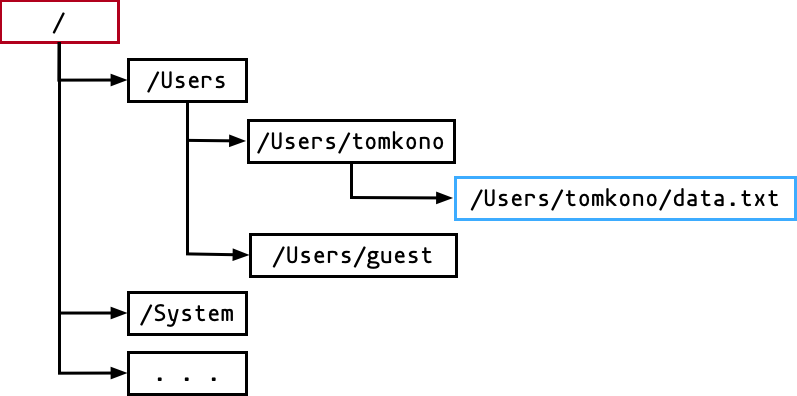
In the tree cartoon above, boxes represent directories or files, and indentation
represents nesting. The text inside the boxes represents the names. The red
box (around /) represents the root of the filesystem, and the blue box
(around /Users/tomkono/data.txt) represents a file. The boxes in black
are directories.
Notice the slashes (/) between parts of the names - these delimit the actual
directories that make up the full path to the file. In the case of
/Users/tomkono/data.txt, you can read the name and know that the file called
data.txt is located under the root (/), then the Users directory, then
the tomkono directory. In UNIX terminology, this is known as the path to
the file. More specifically, it is known as the absolute path because it
starts at the root of the filesystem. This is the way I prefer to specify paths
to files because there is no ambiguity as to where the file is located.
2.1: Basic Commands
We will introduce basic commands briefly, then use them to examine the tutorial’s fastq files.
2.1.1: The Structure of a Command
chaco001@ahl02 [/scratch.global/chaco001] % head -n 100 SRR9327252_1.fastq
A UNIX or Linux command consists of a program, options, and arguments.
-
program (
head): The program is what actually does something to a file. -
options (
-n 100): The options modify the behavior of the program. -
arguments (
SRR9327252_1.fastq): The arguments are the files on which the program operates.
-
commands are case-sensitive!
-
spaces are important!
-
arguments and options are command-specific!
-
one can navigate with keyboard arrows, but not mouse!
2.1.3:Basic Commands
# general basic commands
cd <dest>    change directory to destination
cd ..   go up one directory
cd ~/   go to your home directory
ls    list files
pwd   print working directory
mkdir create a directory
cp <src> <dest>   copy file from src to dest
head <file>    see top lines in file
tail <file>    see bottom lines in file
nano    open file in a text-based file editor
echo <variable>  print the variable in the terminal
zcat <file.gz>  de-compress a gz file
grep <file> <pattern> search for <pattern> within <file>
man <command> get the manual for <command> (alternatively: command --help)
| the pipe operator, puts the results from the command on the left into the command on the right
wc <file> count the number of lines and characters in a file

# MSI-specific commands (mostly from SLURM)
$USER a variable which holds your user ID
echo $USER  show your username
squeue -u $USER show your pending and running jobs
userquota -u $USER  show your current storage quota and usage
module avail <software> see what version of <software> are available
module load <software> load the <software>
2.2: Accessing a Command Line on MSI using Open OnDemand
The following link is to a text file containing all commands run on the command line during this tutorial:
rnaseq_cmd_workshop_commands.txt
Open a web browser and navigate to https://ood.msi.umn.edu/. Log in with your UMN user name and password. You will see a screen like the one shown below:

Click on the Clusters button. A drop-down menu will fold out. Click on
Agate Shell Access:

A new tab will open with a command line prompt.
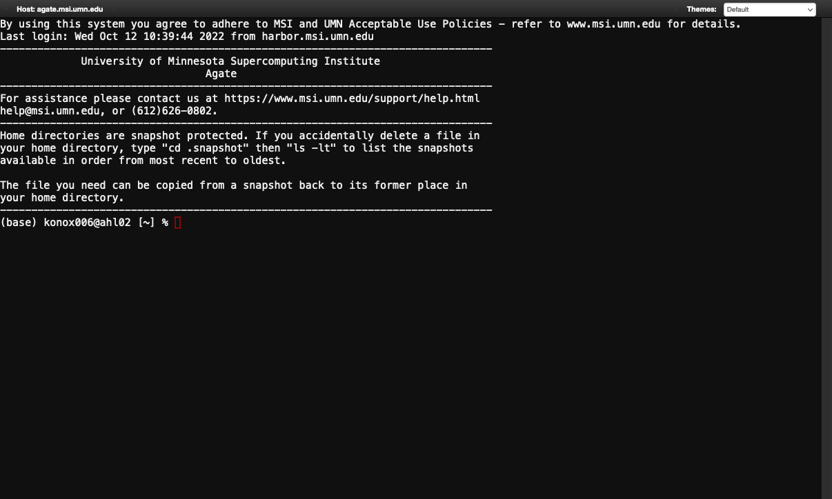
The portion of the prompt to the left of and including the percent symbol (%)
is called the “prompt.” The block is called the “cursor.” When you type
commands into the command line, the symbols will appear to the left of the
cursor:
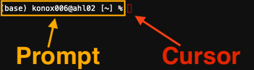
Note that my prompt may look different from yours! The function is identical, regardless of appearance.
Note that you cannot use the mouse to move the cursor around in the terminal area! You must use the arrow keys to move the cursor to edit the command you are currently typing.
2.2.1: Examine fastq files on the command line
We will use the above commands to examine input files and later run CHURP.
First we change directories to where the tutorial files are located.
chaco001@ahl02 [/scratch.global/chaco001] % cd /common/tutorials/bioinformatics/bulk_rnaseq/Reads/
- note that my prompt changed to reflect the new location.
Print the working directory to ensure we are where we expect.
chaco001@ahl02 [/common/tutorials/bioinformatics/bulk_rnaseq/Reads/] % pwd
/common/tutorials/bioinformatics/bulk_rnaseq/Reads/
Next we examine the contents of this directory.
chaco001@ahl02 [/common/tutorials/bioinformatics/bulk_rnaseq/Reads/] % ls

Notes:
- sixteen files
- two per sample
Examine a fastq file. This requires decompressing (zcat), then piping (|)
the results to head (head), so we only look at the top 8 lines (-n 8).
chaco001@ahl02 [/common/tutorials/bioinformatics/bulk_rnaseq/Reads/] % zcat BoneMarrow-1_S23_R1_001.fastq.gz | head -n 8
@SRR7989587:1:TAGCTT:300/1
AGGTGCTCGGCTTCCATTACTGTAGTAGCTGCTGTTCACTGCTCCTTGGCTACCTATGAAATGTTTGATTGAAAATCACT
+SRR7989587.1 1 length=150
AAAAFJAFJFF<FJJAFAJJJJJFJJJFJJJJ<JJFJJJJJJ-FJJJJJJF<77AAFF-FFJFJJJJJJJJFJJFJJJJJ
@SRR7989587:2:TAGCTT:300/1
ATTTTACCAACTGTGTTTTTGTTTTGTTTTGTTTTTTAAGCCACTGCTCAAGTTAATGTCACTGACAGATGGTAAGTTCG
+SRR7989587.2 2 length=150
AA<AFJJJAJJFFAFFJ<FJF-AAJJJFJJJJ<AFJJJJJJFJJJJJFJJJJJFJJJJAJJFJJJJJJJFJJJJF-FFJJ
Notes:
- four lines per read: name (@), sequence, metadata (+), quality score
- no information on genomic location of read! (this is why CHURP requires other files)
Examine that fastq’s partner file (note the “2” in the file name).
chaco001@ahl02 [/common/tutorials/bioinformatics/bulk_rnaseq/Reads/] % zcat \
BoneMarrow-1_S23_R2_001.fastq.gz | head -n 8
@SRR7989587:1:TAGCTT:300/2
GGCAAACAAGTCCAGTTACGGGGGCCCAGCCAGCCAGCAACTGAGAGGGGGTTACGGAAGAGGTTACGGTGGCAAGAGCA
+SRR7989587.1 1 length=150
AAAFFJJ7JJF-<F7--F<-----7F-F--AF--7FF7---7<A<-<F-A7--A-7FA-F-<-77--<AFFA77-77--A
@SRR7989587:2:TAGCTT:300/2
AGCATCCAGCGTTCCAGGAGCCTGGAGAAACCACCACGTATGCACGGGTGGAATCTGAGTTGGACACAAGTGCACTTAAC
+SRR7989587.2 2 length=150
AAAFFJJFJJJJJFJJFJFJ-FFJFJFJJJJJJJJJJFFJJJFJJJJJFJF-AJJAFFFJFJ-7A-FJJAJAJJ<7AAJJ
Do a gut-check: do both fastq files have the same number of reads (=lines)? They should. Pipe the decompressed file into wc with the option (-l) to count the number of lines.
chaco001@ahl02 [/common/tutorials/bioinformatics/bulk_rnaseq/Reads/] % zcat BoneMarrow-1_S23_R1_001.fastq.gz | wc -l
4026016
chaco001@ahl02 [/common/tutorials/bioinformatics/bulk_rnaseq/Reads/] % zcat BoneMarrow-1_S23_R2_001.fastq.gz | wc -l
4026016
3: CHURP Basics
3.1: CHURP sequence analysis overview
At this point we know where the fastq files are
(/common/tutorials/bioinformatics/bulk_rnaseq/Reads/) and how to navigate on MSI, so
we are ready to load CHURP. First I will briefly explain what CHURP does:
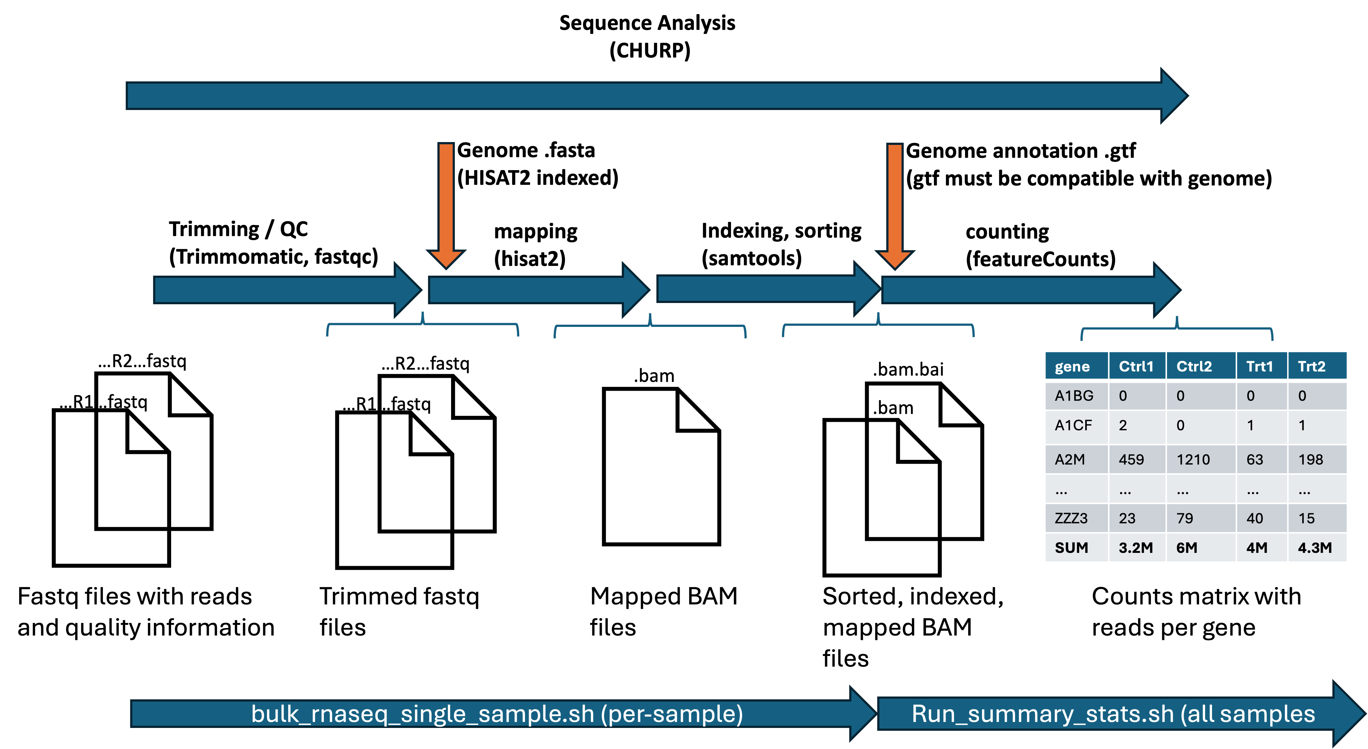
Briefly, the SEQUENCE ANALYSIS steps of the workflow are as follows:
Per-sample:
-
Summarize read quality (
fastqc). -
Clean reads for low-quality bases and adapter contaminants (
trimmomatic). -
Map reads to genome to generate a BAM file (
hisat2). -
Manipulate mapped BAM to right format (
samtools)
(additionally, contamination and complexity are analyzed with bbduk and rnaseqc)
Across all samples:
-
Count reads within genes (
featureCounts). -
Statistical analysis (more details next) (
R, especiallyedgeR). -
Make report (
R).
3.2: CHURP statistical analysis overview
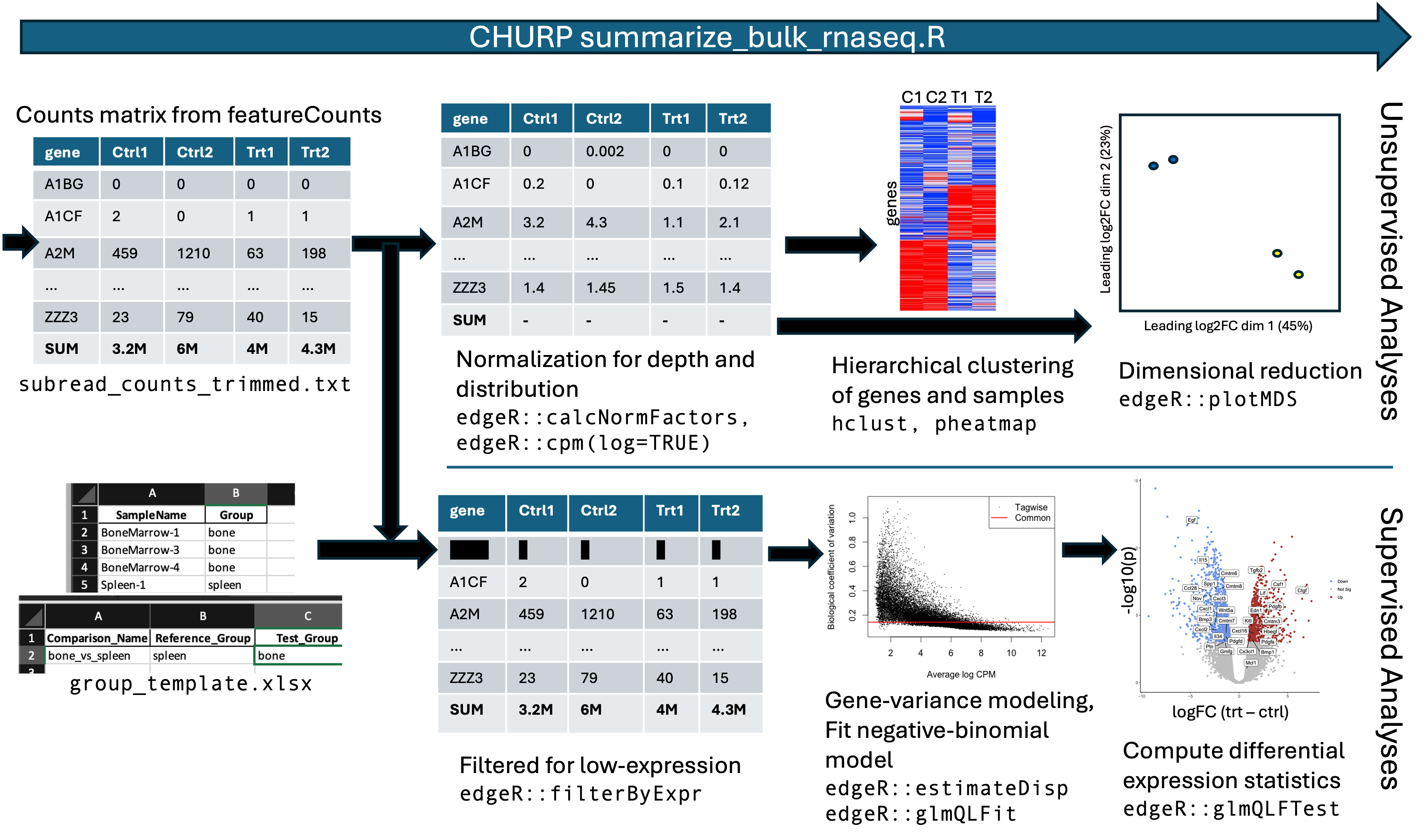
-
This graphic shows the main statistical steps done on the counts matrix.
-
The top row shows the unsupervised analyses which are done on all samples
-
The bottom row shows the supervised analyses done only if comparisons / contrasts were created in the group_template.xlsx (more on that later).
3.3: Accessing and Running CHURP
3.3.1: Using the module system to load CHURP
MSI maintains software for users which can be loaded via module load
Software List: https://msi.umn.edu/our-resources/msi-software
We will access CHURP using module load. We will start from a new directory we make in MSI’s global scratch, which is a special part of the MSI filesystem where you can write temporary data that lasts for one month.
You cannot use my scratch folder (/scratch.global/chaco001) because you do not
have permission to access it. To try to prevent confusion, we will therefore use
the $USER variable whenever I would typically write chaco001 so that your
information is used instead of mine.
The / at the beginning of the file path is important. If you omit it, the
computer will interpret the file path as relative to the current path.
First we check that $USER is working as expected by echoing it, then we move
to our /scratch.global/ folder
chaco001@ahl02 [/common/tutorials/bioinformatics/bulk_rnaseq/Reads/] % echo $USER
chaco001
chaco001@ahl02 [/common/tutorials/bioinformatics/bulk_rnaseq/Reads/] % cd /scratch.global/$USER
chaco001@ahl02 [/scratch.global/chaco001] %
Notes:
- See that my username was returned when
echo $USERwas run. - See that I moved into my scratch directory.
If you do not yet have a /scratch.global/$USER folder, then you will need
to make it with the following code.
Afterwards, you can use cd /scratch.global/$USER to move to the new directory.
chaco001@ahl02 [/common/tutorials/bioinformatics/bulk_rnaseq/Reads/] % mkdir /scratch.global/$USER
**Learn to copy a file here:**
There is no need to copy files in this tutorial but since it is a common command we show the usage here.
Next, we will copy a file into our current directory. We use the cp command
to do this. cp takes two arguments, a source and a destination. For this
exercise, the source will be a long path name:
/projects/standard/riss/public/Pathway_Analysis_Tutorial/Test_Data/Drosophila_melanogaster_edgeR_DEG_table_full.txt
and the destination will be the current working directory. This is
shorthanded by a dot (.) in the command:
chaco001@ahl02 [/scratch.global/chaco001] % cp /projects/standard/riss/public/Pathway_Analysis_Tutorial/Test_Data/Drosophila_melanogaster_edgeR_DEG_table_full.txt .
Once you have done that, you should see the file if you do ls.
Important: long commands can be broken up using backslashes to make it easier to read. We will show CHURP commands like this shortly:
this_is_a_really_long_command_line \
    with_many_options \
    and_with_many_long_arguments \
    such_that_wrapping_makes \
    it_easier_to_read
See what version of churp are available with module avail:
chaco001@ahl02 [/scratch.global/chaco001] % module avail churp
--------------------------------------------
/common/software/modulefiles/migrated/common
--------------------------------------------
churp/0.2.2-slurm  churp/0.2.3  churp/0.2.4  churp/0.2.5  churp/1.0.0  churp/1.1.0
- note: We will only use the latest version.
Load churp with module load:
chaco001@ahl02 [/scratch.global/chaco001] % module load churp/1.1.0
Latest changes: 2024-07-23
- Filtering routines updated, see
https://github.umn.edu/MSI-RIS/CHURP/blob/main/CHANGES.md#modified for details
- '.in_progress' marker files for jobs submitted but not yet completed to
prevent multiple submissions
- 'subread_counts.trimmed.txt' now uses tabs instead of spaces in its header
This is CHURP version 1.1.0.
CHURP can be called by running $CHURP.
chaco001@ahl02 [/scratch.global/chaco001] %
- note: $CHURP runs the program
3.3.2: Try running $CHURP and learn required inputs
See what happens when we run $CHURP:
chaco001@ahl02 [/scratch.global/chaco001] % $CHURP
Usage: churp.py <subcommand> <options>
where <subcommand> is the name of the pipeline that is to be run. The specified
<options> will be applied to the operations in the pipeline. Each pipeline has
its own set of options that must be specified. To see a full listing of each
available option for a given pipeline, pass the '--help' option. Alternately,
online help is maintained at the GitHub repository.
Currently, the following subcommands are supported:
    - group_template
    - bulk_rnaseq
For issues, contact help@msi.umn.edu.
Version: 1.1.0
2024-07-23
chaco001@ahl02 [/scratch.global/chaco001] %
- note: must use a subcommand
- note: the more direct email is ribhelp@msi.umn.edu (help@msi.umn.edu is better for general questions)
See the help for churp’s bulk_rnaseq subcommand:
Note: some output is hard to show using copy/paste so some output is linked images. Furthermore, I have omitted the optional arguments from this for the moment.
chaco001@ahl02 [/scratch.global/chaco001] % $CHURP bulk_rnaseq --help
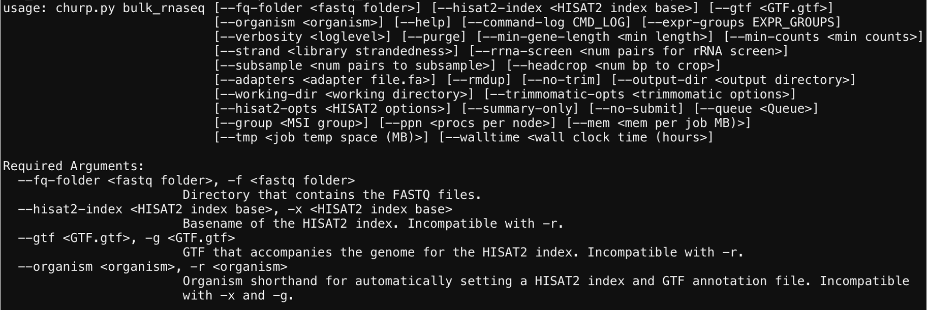
Notes:
-
three required inputs (fq-folder, hisat2-index, gtf)
-
MANY optional arguments (non-standard adapters, downstream filtering, etc.)
CHURP command we are building (must replace ??? with inputs):
$CHURP bulk_rnaseq \
  --fq-folder ??? \
  --hisat2-index ??? \
  --gtf ???
Question: which of these do we already know?
$CHURP bulk_rnaseq \
  --fq-folder /common/tutorials/bioinformatics/bulk_rnaseq/Reads/ \
  --hisat2-index ??? \
  --gtf ???
Other Required Inputs:
-
hisat2-index: pre-made index for the genome hisat2 uses for mapping. Specifically, the basename (directory + file prefix)
-
gtf: “Gene Transfer Format” file for the genome stating gene feature locations. Specifically, a file ending in .gtf
3.3.3: MSI’s bioref database
MSI provides all up-to-date ensembl main indices, gtfs, and other info in /common/bioref/ensembl
The latest information can be found at https://msi.umn.edu/bioref
The main ensembl databases can be found at https://useast.ensembl.org/index.html
Within /common/bioref/ensembl, organisms are split up by taxon / popularity
main: Model organisms and vertebratesgrch37: GRCh37 build of the human genomefungi: Fungimetazoa: Invertebrates and other animalsplants: Green plants and algaeprotists: Organisms colloquially known as “protists”
Recall, our tutorial dataset is analyzing RNA from the house mouse (Mus musculus) which is a model organism.
Navigate to this organism’s databases on MSI and find the paths of the hisat2 index and gtf:
chaco001@ahl02 [/scratch.global/chaco001] % cd /common/bioref/ensembl/main/Mus_musculus-113/GRCm39/
chaco001@ahl02 [/common/bioref/ensembl/main/Mus_musculus-113/GRCm39/] % ls
annotation  blast  bowtie  bowtie2  bwa  hisat2  logs  seq
Note the multiple databases. seq holds the genome, hisat2 holds the index,
and annotation holds the gtf. Examine the sequence fasta:
chaco001@ahl02 [/common/bioref/ensembl/main/Mus_musculus-113/GRCm39/] % cd seq
chaco001@ahl02 [/common/bioref/ensembl/main/Mus_musculus-113/GRCm39/seq] % ls
FASTA.DONE            FASTA_FILE_WGET_LOG     Mus_musculus.GRCm39.dna.toplevel.fa
SAMTOOLS.DONE  genome.fa    FASTA_CKSUM_WGET_LOG
FASTA_REMOTE_CHECKSUMS    Mus_musculus.GRCm39.dna.toplevel.fa.gz  chromlen.len
genome.fa.fai
The genome.fa shows the bases for each chromosome. But it doesn’t show where
genes are!
chaco001@ahl02 [/common/bioref/ensembl/main/Mus_musculus-113/GRCm39/seq] % head -n 2 genome.fa
>1 dna:chromosome chromosome:GRCm39:1:1:195154279:1 REF
NNNNNNNNNNNNNNNNNNNNNNNNNNNNNNNNNNNNNNNNNNNNNNNNNNNNNNNNNNNN
Navigate to the hisat2 directory and examine the contents. The basename is the full directory path, plus the filename part before the #.ht2
# input
chaco001@ahl02 [/common/bioref/ensembl/main/Mus_musculus-113/GRCm39/seq] % cd ..
chaco001@ahl02 [/common/bioref/ensembl/main/Mus_musculus-113/GRCm39] % cd hisat2
chaco001@ahl02 [/common/bioref/ensembl/main/Mus_musculus-113/GRCm39/hisat2] % ls
HISAT2.DONE  genome.1.ht2  genome.2.ht2
genome.3.ht2  genome.4.ht2  genome.5.ht2
genome.6.ht2  genome.7.ht2  genome.8.ht2
Now we know that our hisat2-index is:
/common/bioref/ensembl/main/Mus_musculus-113/GRCm39/hisat2/genome
and therefore our CHURP command is so far:
$CHURP bulk_rnaseq \
  --fq-folder /common/tutorials/bioinformatics/bulk_rnaseq/Reads/ \
  --hisat2-index /common/bioref/ensembl/main/Mus_musculus-113/GRCm39/hisat2/genome \
  --gtf ???
**Some extra info on hisat2-index**
This hisat2-index is reference genome that has been indexed for use with HISAT2. For this tutorial, we will be using a genome index that was prepared specially for the tutorial dataset. For an analysis of a real dataset, you will need to use an index prepared from a full genome assembly. A collection of pre-made indices for MSI users (“bioref,” see Part 3.4) and instructions for making your own indices will not be covered directly as part of this tutorial, but will be described in Supplement 1.
Navigate to the annotation directory and examine the contents. The gtf is the one ending in .gtf.
chaco001@ahl02 [/common/bioref/ensembl/main/Mus_musculus-113/GRCm39/hisat2] % cd ..
chaco001@ahl02 [/common/bioref/ensembl/main/Mus_musculus-113/GRCm39] % cd annotation
chaco001@ahl02 [/common/bioref/ensembl/main/Mus_musculus-113/GRCm39/annotation] % ls
GFF.DONE            GFF_REMOTE_CHECKSUMS  GTF_FILE_WGET_LOG
Mus_musculus.GRCm39.113.gff3.gz   GFF_CKSUM_WGET_LOG  GTF.DONE
GTF_REMOTE_CHECKSUMS          Mus_musculus.GRCm39.113.gtf   GFF_FILE_WGET_LOG
GTF_CKSUM_WGET_LOG    Mus_musculus.GRCm39.113.gff3    Mus_musculus.GRCm39.113.gtf.gz
Now we know that our gtf is:
/common/bioref/ensembl/main/Mus_musculus-113/GRCm39/annotation/Mus_musculus.GRCm39.113.gtf
Look at the head (top lines) of the gtf file to see that it contains gene feature
position information.
chaco001@ahl02 [/common/bioref/ensembl/main/Mus_musculus-113/GRCm39/annotation] % head Mus_musculus.GRCm39.113.gtf
#!genome-build GRCm39
#!genome-version GRCm39
#!genome-date 2020-06
#!genome-build-accession GCA_000001635.9
#!genebuild-last-updated 2023-04
1       havana  gene    108344807       108347562       .       +       .       gene_id "ENSMUSG00000104478"; ...
1       havana  transcript      108344807       108347562       .       +       .       gene_id "ENSMUSG00000104478"; ...
1       havana  exon    108344807       108347562       .       +       .       gene_id "ENSMUSG00000104478"; ...
1       havana  gene    6980784 6981446 .       +       .       gene_id "ENSMUSG00000104385"; ...
1       havana  transcript      6980784 6981446 .       +       .       gene_id "ENSMUSG00000104385"; ...
-
Note: official gtf documentation: https://useast.ensembl.org/info/website/upload/gff.html
-
Note: columns: chrom, source, feature, start, end, score, strand, frame, attribute
I removed most of the attribute column for readability.
CHURP command with all genome information:
$CHURP bulk_rnaseq \
  --fq-folder /common/tutorials/bioinformatics/bulk_rnaseq/Reads/ \
  --hisat2-index "/common/bioref/ensembl/main/Mus_musculus-113/GRCm39/hisat2/genome" \
  --gtf "/common/bioref/ensembl/main/Mus_musculus-113/GRCm39/annotation/Mus_musculus.GRCm39.113.gtf"
**Some extra info on GTF annotations**
CHURP also requires a GTF-formatted file with the gene models annotated on the reference genome. This GTF must match the reference genome that is being used for the HISAT2 index; if the chromosome names or coordinates do not match, then expression levels cannot be accurately estimated. The file can be either gzip-compressed or uncompressed, but like with the FASTQ files, we recommend compression to save disk space.
For this tutorial, we will be using a GTF annotation file that was specially-prepared for use with the HISAT2 index. For an analysis of a real dataset, you will need to use a GTF that comes with a reference genome assembly. bioref contains GTF files that are compatible with the collection of HISAT2 genome indices.
3.3.4: CHURP shortcuts to popular organisms
Notice the –organism “required” option in $CHURP:
CHURP (as of version 0.2.4) includes a genome_aliases subcommand that will
print a table of common genomics models that we maintain in bioref. You can use
these shorthands to automatically specify a reference genome and annotation for
use with CHURP. The table is below:
chaco001@ahl02 [/common/bioref/ensembl/main/Mus_musculus-113/GRCm39/annotation] % $CHURP genome_aliases
Genome Aliases

The species listed in the table below are common genomics models for which we
have provided convenient shortcuts in CHURP. Use the value in the "Alias" column
to automatically set the relevant genome indices and annotation files in other
CHURP pipelines. These names are *case sensitive.* To read more about MSI's
collection of genomics reference data, including the update schedule, please
see the following page:

https://www.msi.umn.edu/content/bioref

The species listed in the table below are common genomics models for which we
have provided convenient shortcuts in CHURP. Use the value in the "Alias" column
to automatically set the relevant genome indices and annotation files in other
CHURP pipelines. These names are *case sensitive.* To read more about MSI's
collection of genomics reference data, including the update schedule, please
see the following page:

https://www.msi.umn.edu/content/bioref

|         Alias | Binomial Name              | Assembly/Annotation             |
|---------------|----------------------------|---------------------------------|
|   arabidopsis | Arabidopsis thaliana       | TAIR10                          |
|        barley | Hordeum vulgare            | MorexV3_pseudomolecules_assembly|
|       chicken | Gallus gallus              | bGalGal1.mat.broiler.GRCg7b     |
| chlamydomonas | Chlamydomonas reinhardtii  | Chlamydomonas_reinhardtii_v5.5  |
|          corn | Zea mays                   | Zm-B73-REFERENCE-NAM-5.0        |
|           cow | Bos taurus                 | ARS-UCD1.2                      |
|           dog | Canis lupus familiaris     | ROS_Cfam_1.0                    |
|           fly | Drosophila melanogaster    | BDGP6.46                        |
|         human | Homo sapiens               | GRCh38.p14                      |
|         mouse | Mus musculus               | GRCm39                          |
|           pig | Sus scrofa                 | Sscrofa11.1                     |
|           rat | Rattus norvegicus          | mRatBN7.2                       |
|    slime_mold | Dictyostelium discoideum   | dicty_2.7                       |
|       soybean | Glycine max                | Glycine_max_v2.1                |
|         wheat | Triticum aestivum          | IWGSC                           |
|          worm | Caenorhabditis elegans     | WBcel235                        |
|         yeast | Saccharomyces cerevisiae   | R64-1-1                         |
|     zebrafish | Danio rerio                | GRCz11                          |
These can be used with the --organism option with CHURP instead of specifying the
--hisat2-index (path to HISAT2 index) and --gtf (path to GTF annotation) values. For
example, these options would be equivalent:
# explicit way
$CHURP bulk_rnaseq \
  --fq-folder /common/tutorials/bioinformatics/bulk_rnaseq/Reads/ \
  --hisat2-index "/common/bioref/ensembl/main/Mus_musculus-113/GRCm39/hisat2/genome" \
  --gtf "/common/bioref/ensembl/main/Mus_musculus-113/GRCm39/annotation/Mus_musculus.GRCm39.113.gtf"

# short cut, same outcome as above
$CHURP bulk_rnaseq \
  --fq-folder /common/tutorials/bioinformatics/bulk_rnaseq/Reads/ \
  --organism mouse
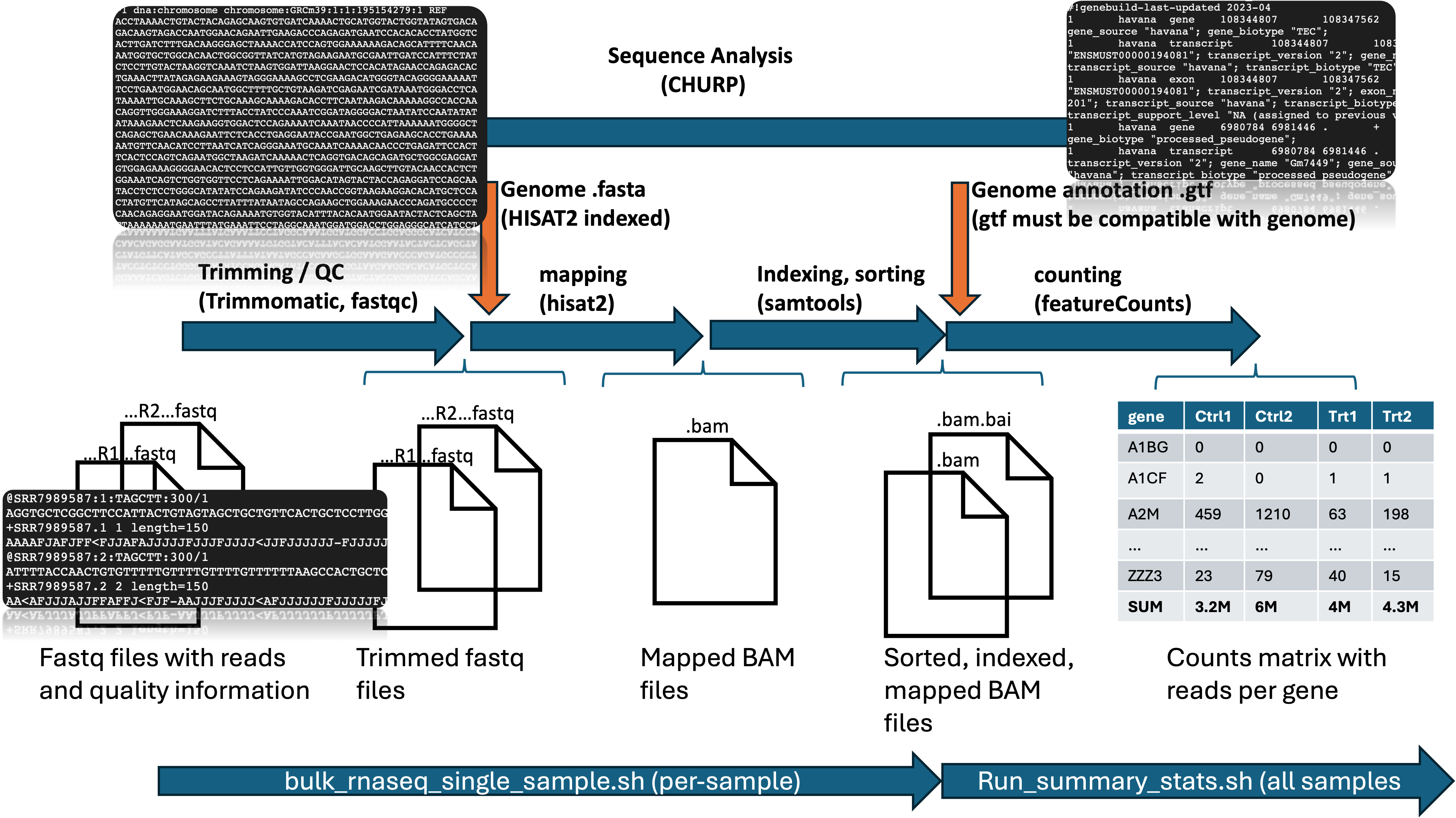
**Graphic of the CHURP pipeline with file snapshots:**
Here is the same pipeline graph as before, but with some snapshots of relevant files to help you connect all the pieces together.
Recall that the left-hand-side of the pipeline is applied to each sample, before summarizing across samples into the counts matrix.
-
Note: The full paths and names of the HISAT2 index and GTF are still printed into the HTML report, so you will have a record of the specific genome and annotation that were used for your analysis.
-
Note: If you can make a good case for another genomics model to be listed in the table, please let us know! The genome must be present in Ensembl and be part of our bioref library.
Part 3.4: Optional - Experimental Groups
- We have not told CHURP which samples belong to which groups
- This information is necessary for differential expression testing, and for plotting group information
- This information is NOT necessary for creating the counts matrix or doing unsupervised analyses
- To provide experimental group metadata, CHURP uses an excel spreadsheet as
an optional input with
--expr-groups
Part 3.4.0: Make a directory for CHURP output
Go back to your /scratch.global/ directory and create a new directory which will hold your output:
chaco001@ahl02 [/common/bioref/ensembl/main/Mus_musculus-113/GRCm39/annotation] % cd /scratch.global/$USER
chaco001@ahl02 [/scratch.global/chaco001] % mkdir RNAseq_Tutorial
chaco001@ahl02 [/scratch.global/chaco001] %
Navigate into that directory:
chaco001@ahl02 [/scratch.global/chaco001] % cd RNAseq_Tutorial
chaco001@ahl02 [/scratch.global/chaco001/RNAseq_Tutorial] %
Part 3.4.1: Using $CHURP group_template to make a fillable excel spreadsheet
Filled-out tutorial groups excel spreadsheet:
https://github.umn.edu/MSI-RIS/Tutorials/blob/gh-pages/tutorial_rnaseq_groups.xlsx
Or use the pre-filled tutorial spreadsheet at this MSI location:
/common/tutorials/bioinformatics/bulk_rnaseq/tutorial_rnaseq_groups.xlsx
The group_template subcommand has it’s own subcommand bulk_rnaseq, upon
which we will call --help:
chaco001@ahl02 [/scratch.global/chaco001/RNAseq_Tutorial] % $CHURP group_template bulk_rnaseq --help
usage: churp.py group_template bulk_rnaseq --fq-folder <fastq folder> [--help] [--verbosity <loglevel>] [--output <output file>] [--command-log CMD_LOG]
Required arguments:
  --fq-folder <fastq folder>, -f <fastq folder>
                        Directory that contains the FASTQ files.
Optional arguments:
  --help, -h            Show this help message and exit.
  --verbosity <loglevel>, -v <loglevel>
                        How much logging output to show. Choose one of "debug,"
                        "info," or "warn."
  --output <output file>, -o <output file>
                        Write the XLSX to this file. Defaults to
                      /scratch.global/chaco001/...bulk_rnaseq.groups.xlsx
  --command-log CMD_LOG
                        Save the command that was run into this file. This file
                        will be appended to, rather than overwritten, so you can
                        save multiple CHURP runs into this file.
Notes:
- required input: fq_folder (
/common/tutorials/bioinformatics/bulk_rnaseq/Reads/) - outputs an xlsx file, by default, in your
/scratch.global/$USERfolder
Make a group_template file in your new folder:
chaco001@ahl02 [/scratch.global/chaco001/RNAseq_Tutorial] % $CHURP group_template bulk_rnaseq \
  --fq-folder /common/tutorials/bioinformatics/bulk_rnaseq/Reads/ \
  --output /scratch.global/$USER/RNAseq_Tutorial/tutorial_rnaseq_groups.xlsx

----------
Thank you for using CHURP. This software was developed by the Research
Informatics Solutions (RIS) group at MSI with funding from the University of
Minnesota Informatics Institute (UMII). For help, please contact
help@msi.umn.edu.
https://www.msi.umn.edu/
https://research.umn.edu/units/umii
----------
SUCCESS
Template file: /scratch.global/chaco001/RNAseq_Tutorial/tutorial_rnaseq_groups.xlsx
All sample groups and any additional columns have specified have been filled
with NULL. Please edit the file and write in the correct values for your
dataset. Samples with the same "Group" label will be treated as replicates
in the analysis. Samples with a "Group" value of NULL will not be used in
downstream differential expression analysis. When you have edited the file to
your liking, supply its path to the "bulk_rnaseq" pipeline with the -e
option to enable group testing.
chaco001@ahl02 [/scratch.global/chaco001] %
We see SUCCESS and the path to the template file.
Part 3.4.2: Edit the group_template xlsx
The easiest way to edit the group template file is to download it, open it in excel (or open office / libre office), save it, then re-upload it.
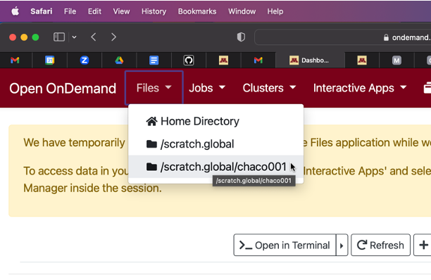
First navigate to the files tab, specifically /scratch.global/$USER:
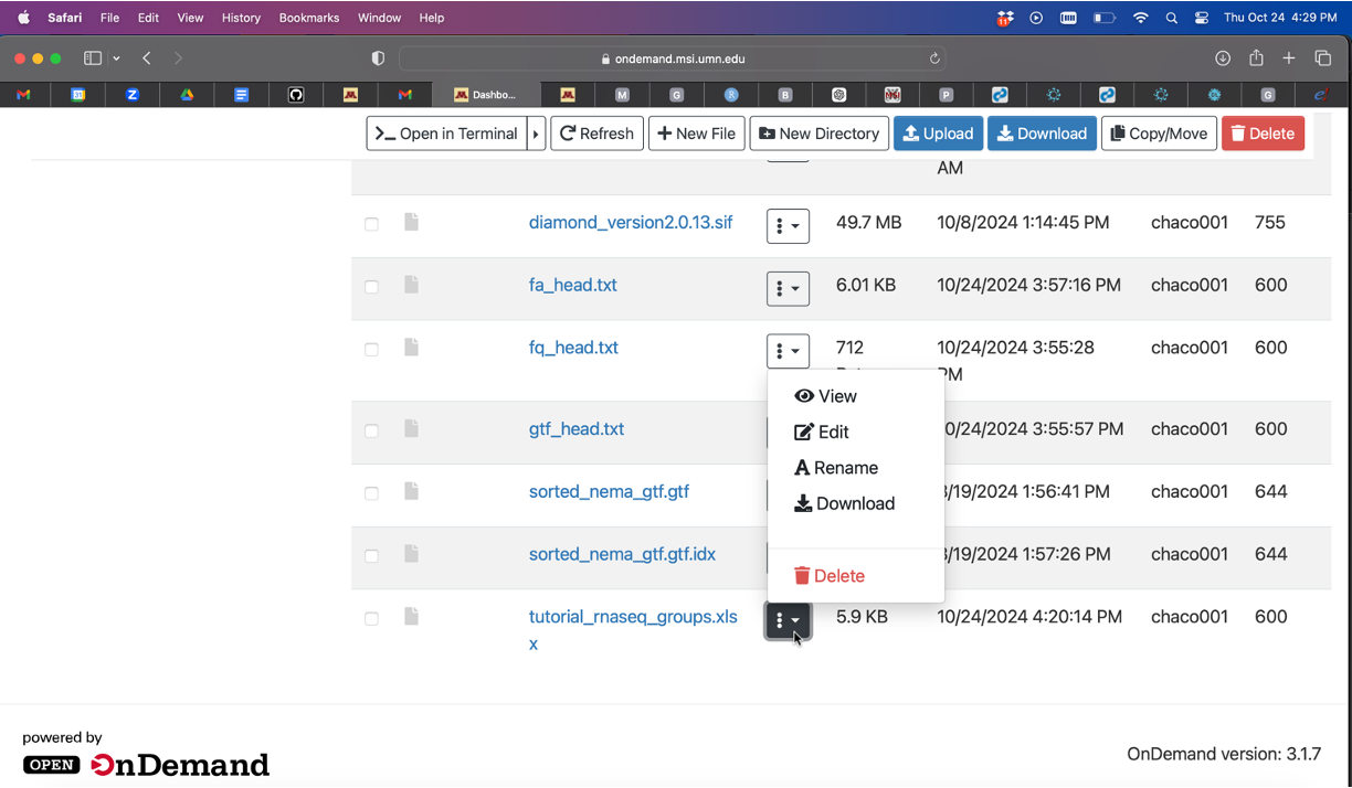
Find the xlsx, then download it:
Open the xlsx and edit the “groups” tab:
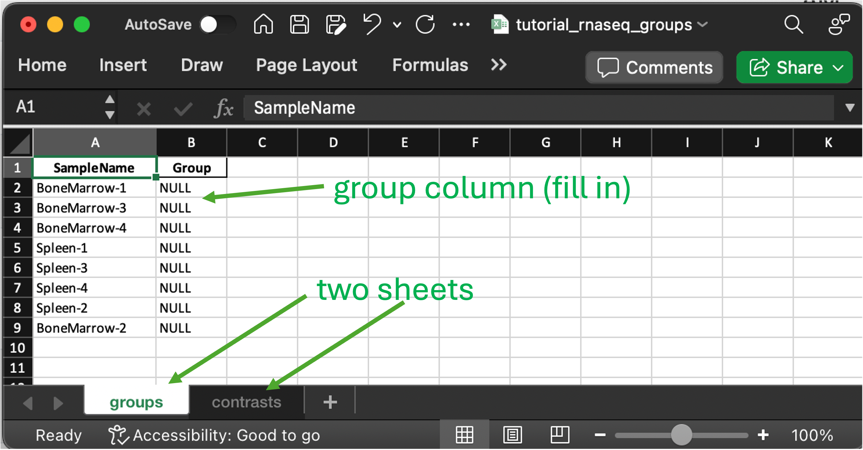
Steps:
-
fill in the group for each sample
-
optionally, add a column called “batch” that will be shown on the MDS plots
-
Note: the “group” designation affects plotting color in the heatmap and MDS plot
Optionally edit the “contrasts” tab:
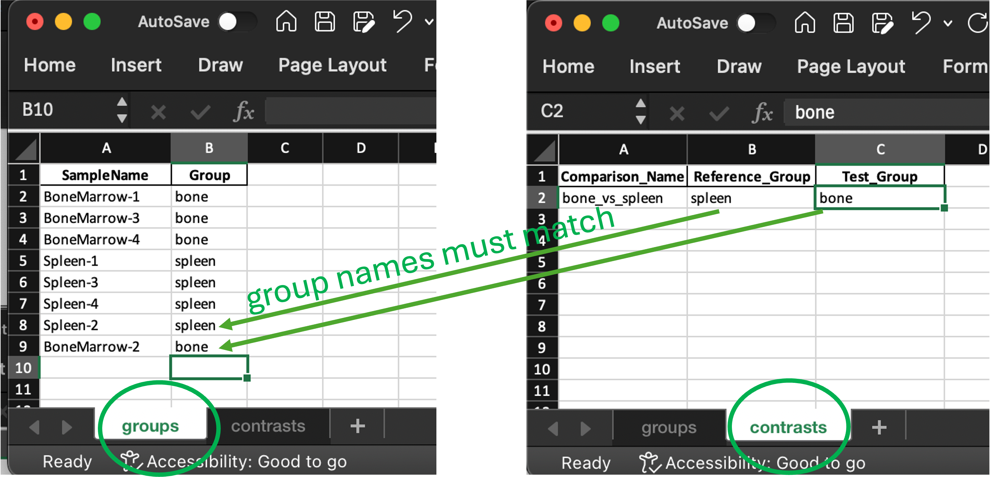
Steps:
-
make a row for each differential expression contrast (“Comparison_Name”) you want to have calculated
-
contrast “Comparison_Names” must be unique.
-
group names must match between sheets.
-
Reference Group is the denominator, Test Group is the numerator
Save the file and upload back in the same directory:
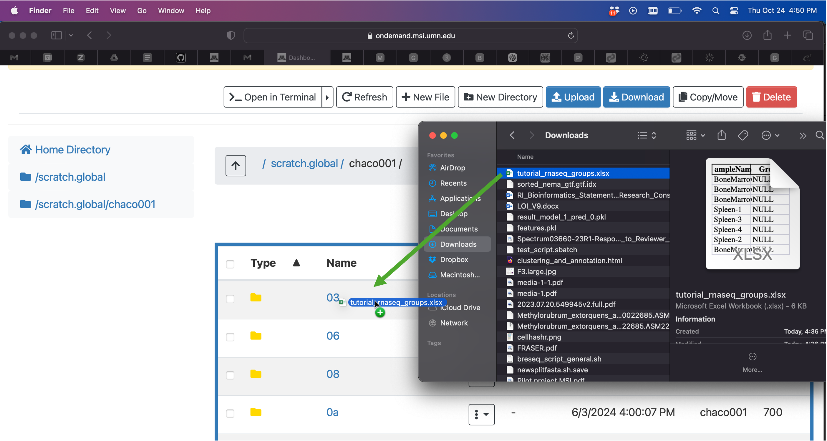
CHURP command with experimental groups (using the pre-made xlsx in /common/):
$CHURP bulk_rnaseq \
  --fq-folder /common/tutorials/bioinformatics/bulk_rnaseq/Reads/ \
  --hisat2-index "/common/bioref/ensembl/main/Mus_musculus-113/GRCm39/hisat2/genome" \
  --gtf "/common/bioref/ensembl/main/Mus_musculus-113/GRCm39/annotation/Mus_musculus.GRCm39.113.gtf"
  --expr-groups "/common/tutorials/bioinformatics/bulk_rnaseq/tutorial_rnaseq_groups.xlsx"
Some extra details on expression groups
CHURP allows you to specify additional metadata columns with the -e option.
This option can be specified multiple times for multiple columns; for example,
to add columns for Age and Sex, you can include -e Age -e Sex in the
command. This makes it easy to build a metadata CSV that can accommodate a more
complicated experimental design. Our automated testing, however, only considers
the Group column. For analysis of more complicated experiments, please
consult with a statistician or with us at RI Bioinformatics!
Note that if you give a sample a NULL group assignment, then it will not
be used for differential gene expression testing. You will still get expression
counts and QC metrics, though.
CHURP will perform automated differential gene expression testing with up to four groups maximum. It will also only perform automated differential expression testing if and only if all groups have at least three replicates. If your experiment does not conform to these parameters, then you will have to perform differential expression testing yourself with the expression matrix produced by CHURP.
Part 3.5: Submit CHURP and checking job
Part 3.5.1: Submitting CHURP and checking created files
We have defined all required inputs and created a group_template.xlsx which is
uploaded to /scratch.global/$USER/RNAseq_Tutorial/tutorial_rnaseq_groups.
It is time to submit CHURP.
Two-step submission: We will submit CHURP in two steps by using the
--no-submit option. This lets us examine the sample sheet to ensure it looks
correct before actually running CHURP. In theory, one can submit CHURP in one
step (by omitting --no-submit) but doing so is less careful.
While we have defined all required arguments to CHURP (fq-folders, gtf, hisat2-index), we will also use a number of optional arguments. Most of these arguments change the job submission settings to reduce the duration of the job, making it likelier to complete during the tutorial. One option is needed to ensure the biology is correctly captured.
CHURP full call with --no-submit`
$CHURP bulk_rnaseq \
  --fq-folder /common/tutorials/bioinformatics/bulk_rnaseq/Reads/ \
  --organism mouse \
  --expr-groups /common/tutorials/bioinformatics/bulk_rnaseq/tutorial_rnaseq_groups.xlsx \
  --output-dir /scratch.global/$USER/RNAseq_Tutorial/Out \
  --working-dir /scratch.global/$USER/RNAseq_Tutorial/Work \
  --strand U \
  --queue msismall \
  --ppn 8 --mem 24000 --walltime 2 \
  --no-submit
The parameters specified here are specific for the tutorial dataset! Do not
re-use these for an analysis of a real dataset! In particular, the --ppn 8
and -w 2 parameters are for extremely small datasets, and the --strand U
parameter is for a specific type of library preparation.
The default RNAseq library preparation kit used by the UMGC is the Illumina
TruSeq Stranded mRNA kit, which uses RF strand specificity. This means R1
maps to the “reverse” strand and R2 maps to the “forward” strand. This is
the default strand specificity for CHURP.
For low input or marginal quality RNA, the UMGC may use the SMARTer Stranded
RNAseq v2 kit from Takara Bio. This kit also has RF strand specificity,
but requires a “headcrop” of 3bp (--headcrop 3 for CHURP).
If you have older data that was from the SMARTer Stranded RNAseq v1 kit, it has
FR strand specificity, and also requires --headcrop 3 for CHURP.
Your data release email from UMGC will specify which kit was used to prepare
your libraries. If you are analyzing data from other sources, you will have to
consult the manual of the kit that was used to prepare your data to know the
strand specificity. The libraries used in this tutorial come from the “NEBNext
Ultra RNA,” which is not strand-specific, which is why we use --strand U
in the tutorial.
Telling CHURP the strand specificity does not affect read mapping; it only affects the way fragments are assigned to genes during the quantification step.
Explanation of the additional arguments:
# Important for our biology:
--strand #our data are unstranded so we specify U

# Not necessary, but helpful:
--output-dir / --working-dir #where final / in-progress files go
--queue # which MSI partition to send the jobs to
--ppn # processors per node
--mem # memory in megabytes per processor
--walltime # how long in hours the jobs can take

# remember, use this to see all arguments:
$CHURP bulk_rnaseq --help
Run the above --no-submit code to generate input files:
chaco001@ahl02 [/scratch.global/chaco001/RNAseq_Tutorial] % $CHURP bulk_rnaseq \
  --fq-folder /common/tutorials/bioinformatics/bulk_rnaseq/Reads/ \
  --organism mouse \
  --expr-groups /common/tutorials/bioinformatics/bulk_rnaseq/tutorial_rnaseq_groups.xlsx \
  --output-dir /scratch.global/$USER/RNAseq_Tutorial/Out \
  --working-dir /scratch.global/$USER/RNAseq_Tutorial/Work \
  --strand U \
  --queue msismall \
  --ppn 8 --mem 24000 --walltime 2 \
  --no-submit
2024-10-30 08:59:11,720 - CHURPipelines.Pipelines.Pipeline - WARNING: Output dir /scratch.global/chaco001/RNAseq_Tutorial/
Out is not empty! Results may be clobbered.
2024-10-30 08:59:11,721 - CHURPipelines.Pipelines.Pipeline - WARNING: Working dir /scratch.global/chaco001/RNAseq_Tutorial
/Work is not empty!
----------
Thank you for using CHURP. This software was developed by the Research
Informatics Solutions (RIS) group at MSI with funding from the University of
Minnesota Informatics Institute (UMII). For help, please contact
help@msi.umn.edu.
https://www.msi.umn.edu/
https://research.umn.edu/units/umii
----------
SUCCESS
Samplesheet and pipeline script generation complete! Their paths are given
below:
Pipeline script: /scratch.global/chaco001/RNAseq_Tutorial/Out/2024-10-30.chaco001.bulk_rnaseq.pipeline.sh
Samplesheet: /scratch.global/chaco001/RNAseq_Tutorial/Out/2024-10-30.chaco001.bulk_rnaseq.samplesheet.txt
Sbatch array key: /scratch.global/chaco001/RNAseq_Tutorial/Out/2024-10-30.chaco001.bulk_rnaseq.qsub_array.txt
Verify the information in the samplesheet, and run the pipeline script with
bash while logged into Mesabi. You will recieve email notifications of job
start/completion/error at your UMN X500 email address. If you need to submit
an error report, please contact help[at]msi.umn.edu. Please include the
samplesheet, pipeline script, and the error message with your report.
chaco001@ahl03 [/scratch.global/chaco001/RNAseq_Tutorial/Out] %
Explanation of output:
Warnings appear because I’d previously run this tutorial, you likely have warnings appear stating that output directories were created.
The important pieces of information are the three paths to files created.
Notice that the message tells you to verify the information in the samplesheet, then run the pipeline script with bash. There is also an outdated reference to Mesabi (a previous version of our supercomputer) which should be ignored.
We will check the sample sheet because that will help us ensure that the groups have been set and that the correct sample name goes with the right fastqs.
Navigate to the Out directory and list the files:
chaco001@ahl02 [/scratch.global/chaco001/RNAseq_Tutorial] % cd Out
chaco001@ahl02 [/scratch.global/chaco001/RNAseq_Tutorial/Out] % ls
2024-10-25.chaco001.bulk_rnaseq.pipeline.sh
2024-10-25.chaco001.bulk_rnaseq.samplesheet.txt  2024-10-25.chaco001.bulk_rnaseq.qsub_array.txt
We see the files we expected to see. What are these files?
2024-10-25.chaco001.bulk_rnaseq.samplesheet.txt: the file we will use to ensure the right settings were applied2024-10-25.chaco001.bulk_rnaseq.qsub_array.txt: a file which links sample names to slurm job submission details (not necessary for users to examine)2024-10-25.chaco001.bulk_rnaseq.pipeline.sh: the actual pipeline file. Useful to understand the internals of CHURP (or modify for bespoke purposes) but not necessary to examine.
Check the sample sheet. We will again use the head command to do this:
The following command MUST be changed to match the sample sheet in your directory, because both the date and the username will be different.
chaco001@ahl02 [/scratch.global/chaco001/RNAseq_Tutorial/Out] % head -n 2 2024-10-25.chaco001.bulk_rnaseq.samplesheet.txt
BoneMarrow-1|bone|/common/tutorials/bioinformatics/bulk_rnaseq/Reads//BoneMarrow-1_S23_R1_001.fastq.gz|/common/tutorials/b
ioinformatics/bulk_rnaseq/Reads//BoneMarrow-1_S23_R2_001.fastq.gz|/scratch.global/chaco001/RNAseq_Tutorial/Out
|/scratch.global/chaco001/RNAseq_Tutorial/Work|yes|no|ILLUMINACLIP:/home/msistaff/public/CHURP_Deps/v1/db/all_illumina_ada
pters.fa:4:15:7:2:true LEADING:3 TRAILING:3 SLIDINGWINDOW:4:15 MINLEN:18|/common/bioref/ensembl/main/Mus_musculus-113/GRCm
39/hisat2/genome|-p 8 --no-mixed --new-summary |0|/common/bioref/ensembl/main/Mus_musculus-113/GRCm39/annotation/Mus_muscu
lus.GRCm39.113.gtf
BoneMarrow-2|bone|/common/tutorials/bioinformatics/bulk_rnaseq/Reads//BoneMarrow-2_S21_R1_001.fastq.gz|/common/tutorials/b
ioinformatics/bulk_rnaseq/Reads//BoneMarrow-2_S21_R2_001.fastq.gz|/scratch.global/chaco001/RNAseq_Tutorial/Out
|/scratch.global/chaco001/RNAseq_Tutorial/Work|yes|no|ILLUMINACLIP:/home/msistaff/public/CHURP_Deps/v1/db/all_illumina_ada
pters.fa:4:15:7:2:true LEADING:3 TRAILING:3 SLIDINGWINDOW:4:15 MINLEN:18|/common/bioref/ensembl/main/Mus_musculus-113/GRCm
39/hisat2/genome|-p 8 --no-mixed --new-summary |0|/common/bioref/ensembl/main/Mus_musculus-113/GRCm39/annotation/Mus_muscu
lus.GRCm39.113.gtf
| Notice the important information, which is separated by “ | ” |
-
each row is a sample.
-
The samples should have the correct group and the right fastqs
-
all samples should have the same genome / annotation files, which should be correct
-
There is also information on the trimmomatic settings (ILLUMINACLIP:/home/msistaff/public/CHURP_Deps/v1/db/all_illumina_ada pters.fa:4:15:7:2:true LEADING:3 TRAILING:3 SLIDINGWINDOW:4:15 MINLEN:18)
Also check that the right number of samples are set to be processed
using wc:
chaco001@ahl02 [/scratch.global/chaco001/RNAseq_Tutorial/Out] % wc -l 2024-10-25.chaco001.bulk_rnaseq.samplesheet.txt
8
If everything seems correct, submit the jobs to be processed on the supercomputer.
This is done by running bash on the file ending in pipeline.sh:
chaco001@ahl03 [/scratch.global/chaco001/RNAseq_Tutorial/Out] % bash 2024-10-30.chaco001.bulk_rnaseq.pipeline.sh
sbatch: Setting account: riss
sbatch: Setting account: riss
You are running CHURP version 1.1.0
Output and logs will be written to /scratch.global/chaco001/RNAseq_Tutorial/Out
Emails will be sent to chaco001@umn.edu
Sbatch array to samplename key: /scratch.global/chaco001/RNAseq_Tutorial/Out/2024-10-30.chaco001.bulk_rnaseq.qsub_array.txt
Single samples job array ID: 25488518
Summary job ID: 25488519
chaco001@ahl03 [/scratch.global/chaco001/RNAseq_Tutorial/Out] %
Important information in output:
-
Shows the CHURP version (should be what you
module loaded) -
Shows the directory into which results will be written
-
Shows to what email job statuses will be sent
-
Shows the ID of the jobs in the job scheduler
Part 3.5.2: Checking the job status in the queue
Once CHURP has been submitted, we can check the jobs’ statuses in the queue.
Note that CHURP makes as many jobs as there are samples, plus one. This is because each sample is processed into a BAM file in its own job, then the counts matrix and report is made in a separate job.
Use squeue to check job status. Your job numbers and user will differ:
chaco001@ahl02 [/scratch.global/chaco001/RNAseq_Tutorial] % squeue -u $USER
             JOBID PARTITION     NAME     USER ST       TIME  NODES NODELIST(REASON)
          25488519   msismall run_summ chaco001 PD       0:00      1 (Dependency)
    25488518_[1-8]   msismall bulk_rna chaco001 PD       0:00      1 (None)
chaco001@ahl02 [/scratch.global/chaco001/RNAseq_Tutorial] %
Notes:
-
we entered your MSI username after
-uusing the $USER variable -
observe the
PARTITIONcolumn matches what we asked for in$CHURP -
observe the
JOBIDmatches the output from$CHURP -
the
ST(status) column will change when the job runs or stops, or is stuck for another reason
Here, I captured the job status before they began running.
Part 4: CHURP output
If your jobs have finished successfully you should have received emails giving
that status. Specifically, the job with a name similar to run_summary_stats.sh
must have completed with SUCCESS for all results to be observed.
Examine the files and directories created by CHURP:
chaco001@ahl03 [/scratch.global/chaco001/RNAseq_Tutorial/Out] % ls
2024-10-25.chaco001.bulk_rnaseq.pipeline.sh
2024-10-25.chaco001.bulk_rnaseq.qsub_array.txt
2024-10-25.chaco001.bulk_rnaseq.samplesheet.txt
Bulk_RNAseq_Report.html
Coordinate_Sorted_BAMs
Counts
Counts.zip
DEGs
InsertSizeMetrics
Logs
Mus_musculus.GRCm39.113.gtf
Plots
allsamples_work_directory
bulk_rnaseq_single_sample-25492402.1.err
bulk_rnaseq_single_sample-25492402.1.out
bulk_rnaseq_single_sample-25492402.2.err
bulk_rnaseq_single_sample-25492402.2.out
bulk_rnaseq_single_sample-25492402.3.err
bulk_rnaseq_single_sample-25492402.3.out
bulk_rnaseq_single_sample-25492402.4.err
bulk_rnaseq_single_sample-25492402.4.out
bulk_rnaseq_single_sample-25492402.5.err
bulk_rnaseq_single_sample-25492402.5.out
bulk_rnaseq_single_sample-25492402.6.err
bulk_rnaseq_single_sample-25492402.6.out
bulk_rnaseq_single_sample-25492402.7.err
bulk_rnaseq_single_sample-25492402.7.out
bulk_rnaseq_single_sample-25492402.8.err
bulk_rnaseq_single_sample-25492402.8.out
gene_id_gene_name_map.txt
run_summary_stats-25492403.err
run_summary_stats-25492403.out
singlesamples_work_directory
Notes:
-
.err and .out files for each job
- output directories:
- Counts, DEGs (if comparisons added to group_template), Logs, Plots, Coordinate_Sorted_BAMs, InsertSizeMetrics (if using paired reads)
- An html report called
Bulk_RNAseq_Report.html
Part 4.1: CHURP BAM files
Most results are easiest to examine using the Open OnDemand browser. The exception are the BAM files. These are the files which show the coordinates to which each read mapped, and many important mapping details. While one doesn’t need to understand them to use CHURP or do differential expression testing, it is good to familiarize oneself with them as they are the basis for many other workflows.
These files cannot be viewed with Open OnDemand because they are compressed, and therefore special software is required. Luckily we have a module for that!
Navigate to the Coordinate_Sorted_BAMs directory and list what files are present:
chaco001@ahl02 [/scratch.global/chaco001/RNAseq_Tutorial] % cd Coordinate_Sorted_BAMs
chaco001@ahl02 [/scratch.global/chaco001/RNAseq_Tutorial/Coordinate_Sorted_BAMs] % ls
BoneMarrow-1_MAPQFiltered_CoordSort.bam      Spleen-1_MAPQFiltered_CoordSort.bam
BoneMarrow-1_MAPQFiltered_CoordSort.bam.bai  Spleen-1_MAPQFiltered_CoordSort.bam.bai
BoneMarrow-1_Raw_CoordSort.bam               Spleen-1_Raw_CoordSort.bam
BoneMarrow-1_Raw_CoordSort.bam.bai           Spleen-1_Raw_CoordSort.bam.bai
BoneMarrow-2_MAPQFiltered_CoordSort.bam      Spleen-2_MAPQFiltered_CoordSort.bam
BoneMarrow-2_MAPQFiltered_CoordSort.bam.bai  Spleen-2_MAPQFiltered_CoordSort.bam.bai
BoneMarrow-2_Raw_CoordSort.bam               Spleen-2_Raw_CoordSort.bam
BoneMarrow-2_Raw_CoordSort.bam.bai           Spleen-2_Raw_CoordSort.bam.bai
BoneMarrow-3_MAPQFiltered_CoordSort.bam      Spleen-3_MAPQFiltered_CoordSort.bam
BoneMarrow-3_MAPQFiltered_CoordSort.bam.bai  Spleen-3_MAPQFiltered_CoordSort.bam.bai
BoneMarrow-3_Raw_CoordSort.bam               Spleen-3_Raw_CoordSort.bam
BoneMarrow-3_Raw_CoordSort.bam.bai           Spleen-3_Raw_CoordSort.bam.bai
BoneMarrow-4_MAPQFiltered_CoordSort.bam      Spleen-4_MAPQFiltered_CoordSort.bam
BoneMarrow-4_MAPQFiltered_CoordSort.bam.bai  Spleen-4_MAPQFiltered_CoordSort.bam.bai
BoneMarrow-4_Raw_CoordSort.bam               Spleen-4_Raw_CoordSort.bam
BoneMarrow-4_Raw_CoordSort.bam.bai           Spleen-4_Raw_CoordSort.bam.bai
There is a filtered and unfiltered BAM per sample, as well as an index (.bai).
We will use samtools, a common and useful bioinformatics tool, to decompress
one BAM file and look at its head.
chaco001@ahl02 [/scratch.global/chaco001/RNAseq_Tutorial/Coordinate_Sorted_BAMs] % module load samtools/1.16.1-gcc-8.2.0-egljrr3
chaco001@ahl02 [/scratch.global/chaco001/RNAseq_Tutorial/Coordinate_Sorted_BAMs] % samtools view BoneMarrow-1_MAPQFiltered_CoordSort.bam | head -3
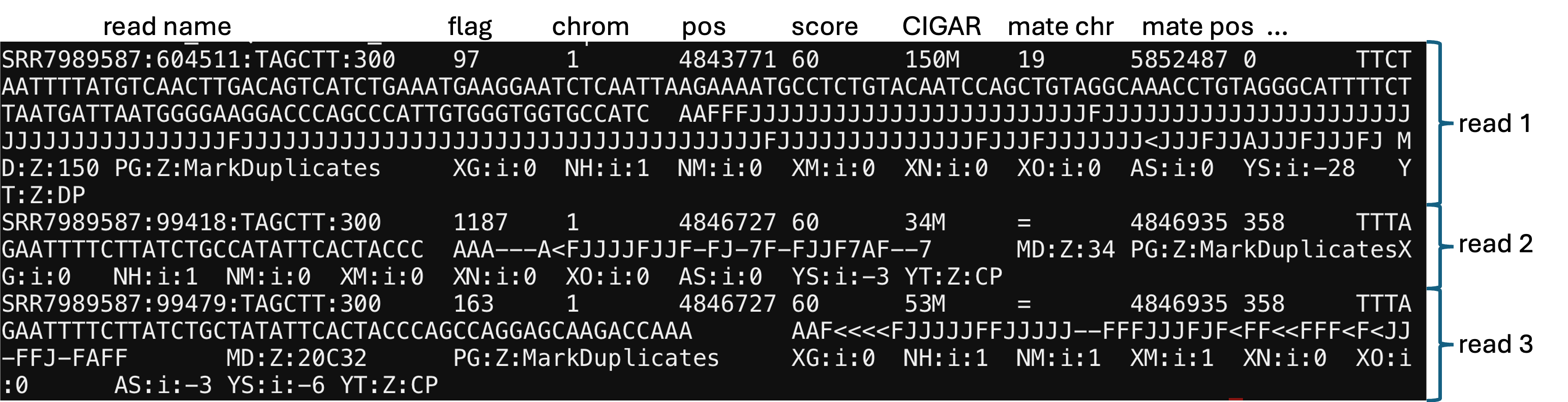
-
This is the first three rows. The first column is the read name, then mapping flag, chromosome name, chromosome position, mapping score, CIGAR score, mate reference name, mate position, template length, sequence, Phred score, and then additional columns with alignment information. See Hisat2 instructions for specifics.
-
This file can be visualized using IGV to see read pileups and variants. (IGV is on Open OnDemand!)
-
This file can be used for other analyses such as differential splicing.
Part 4.2: CHURP output directories
Navigate to the output directory on Open OnDemand to peruse the remaining outputs:
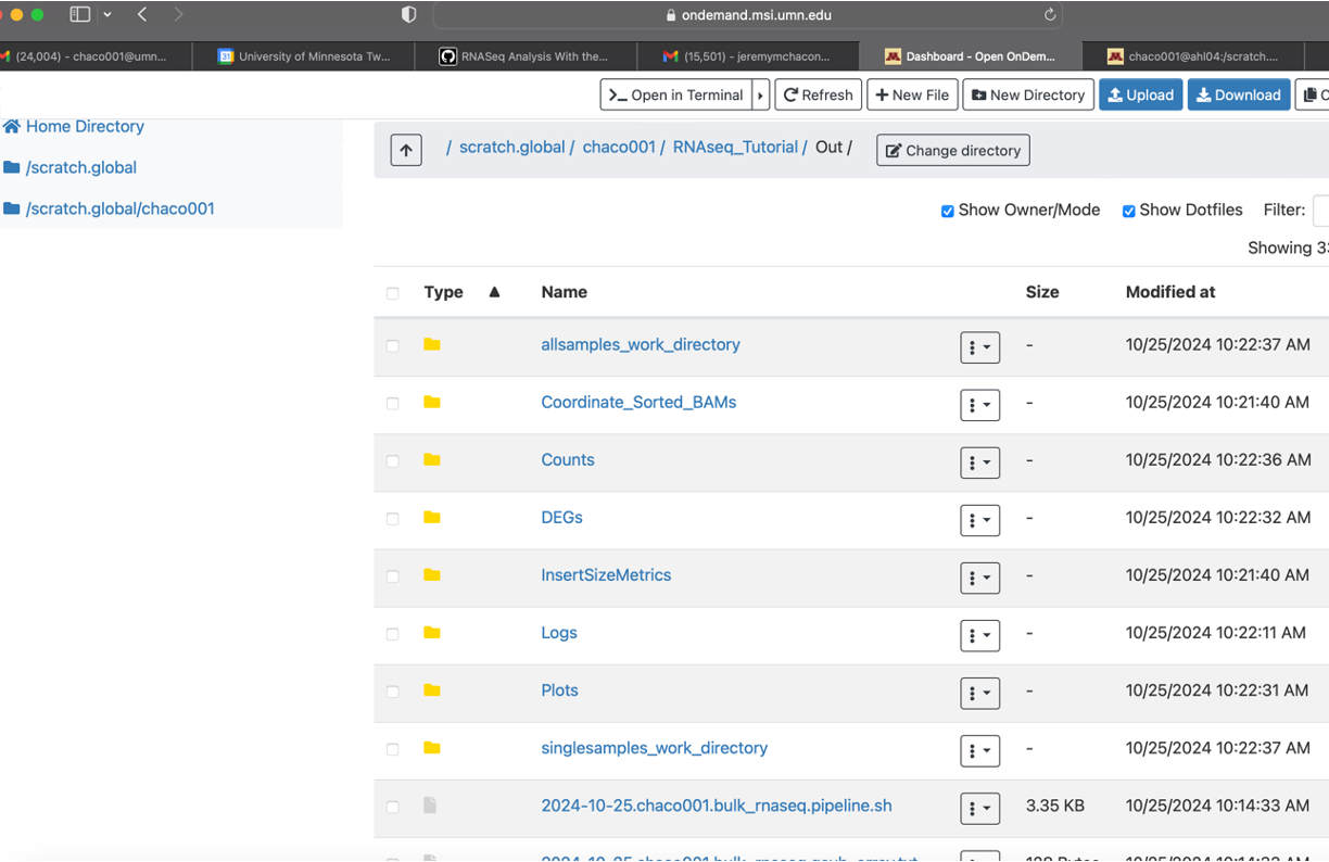
Part 4.2.1: CHURP most important directories
We will focus here on the most important directories.
Navigate into the Counts directory and observe the outputs:
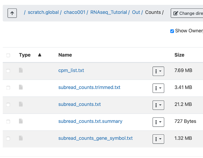
Notes:
-
These files contain counts matrices that have one gene per row and the samples are columns. They can be loaded into R or other programs for re-analysis.
-
subread_counts_trimmed.txtis the main file to use for re-analysis as it omits extraneous transcript metadata in subread_counts.txt. The values in the cells are the raw read counts. -
featureCounts created
subread_counts.txtfrom which all other files derive -
cpm_list.txtcontains filtered and normalized counts in “log base 2 counts per-million” values. This should only be used for visualization, not statistical analysis. -
subread_counts_gene_symbol.txtis the same assubread_counts_trimmed.txtbut with human-readable gene symbols rather than stable gene IDs. This file may be easiest to open and look through in Excel.
Snippet showing loading raw read counts into R
We will not perform any analysis with subread_counts_trimmed.txt directly,
least of all with a text file viewer. This is outside of the scope of this
tutorial, but if you would like to read these values into R, you can use the
following snippet:
subread_cts <- read.table("subread_counts_trimmed.txt", header=TRUE, sep="\t")
raw_read_cts <- as.matrix(subread_cts[,-c(1:6)])
rownames(raw_read_cts) <- subread_cts[, 1]
Note: you will need to specify the path as well in read.table(), or copy the txt file to your working directory.
These can then be used as the expression data for analysis with EdgeR or DESeq2. If you are interested in performing your own differential expression analysis, then you can refer to the guides for EdgeR and DESeq2:
- EdgeR: http://bioconductor.org/packages/release/bioc/html/edgeR.html
- DESeq2: https://bioconductor.org/packages/release/bioc/html/DESeq2.html
The experimental metadata CSV that you generated will also be helpful for running your own differential expression analyses.
Navigate to the DEGs directory:
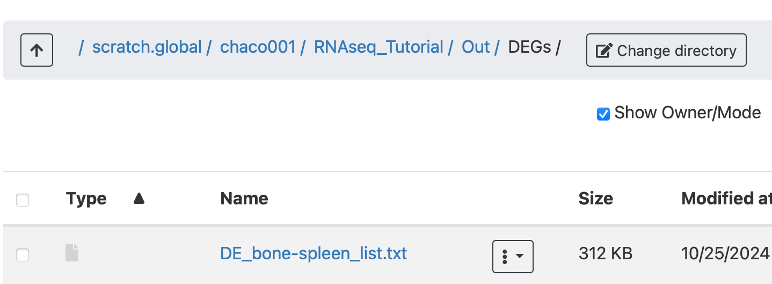
Understand DEG file names with respect to reference / test groups
The filename has some interpretative meaning here. You will notice that the
filename has a pair of the group names that we assigned in Part 4.2, in
this case Spleen and BoneMarrow. These denote the groups that were compared
for differential gene expression.
The general form the filename takes is DE_GROUP2-GROUP1_list.txt, and GROUP1
is treated as the reference group and GROUP2 is treated as the test group.
Therefore, genes that have positive log(fold change) values
are up-regulated in GROUP2 with respect to GROUP1, and genes
with negative log(fold change) values are down-regulated in GROUP2 with
respect to GROUP1. In this case, BoneMarrow is the reference group, and
Spleen is the test group.
These are main outputs if you designated differential expression comparisons to be made. We specified one contrast, so there is one file. Click it:

The first row has the names of the columns. There are six pieces of information for each gene:
genes:gene namelogFC:log2(fold change) test group - reference grouplogCPM:average log2(expression) over all samples in matrixF:Ftest statistic from quasi-likelihood edgeR analysisPvalue:raw p-value for the test statisticFDR:BH-corrected p-value to adjust for multiple comparisons
Traditionally, “differentially-expressed genes” are those with FDR < 0.05 AND absolute(logFC) > 1, but these thresholds depend on the experiment.
Details on filtering done before testing
The test that is done is the quasi-likelihood F test in EdgeR. You can read
more about the quasi-likelihood F test in the EdgeR user manual:
https://bioconductor.org/packages/release/bioc/html/edgeR.html
The expression values are filtered before being used for differential gene expression testing with CHURP. The following filters are applied:
- Genes that are shorter than 200bp are removed (this can be adjusted with a command line argument).
- Samples with
NULLgroup assignments are removed. - Genes with low expression* are removed.
*: We define “low expression” as follows:
- Calculate the median library size.
- Calculate
C, the CPM (not on the log2 scale) value that would be obtained from a raw count ofXfragments in this median library. By defaultXis 10 fragments, but is adjustable with the--min-countoption to CHURP. - Calculate
K, the size of the smallest non-NULLgroup. - Calculate CPM (not log2 scale) for all genes in non-
NULLsamples. - Keep only genes where at least
Ksamples have an expression level ofCor greater, regardless of their group assignment.
This filtering scheme is similar to that implemented by edgeR’s
filterByExpr() function. We recreate it manually so that we can fully report
the calculated thresholds for sample number and expression level.
We still advocate that differential expression testing be done with human input, rather than with the automated processing. CHURP cannot automatically evaluate diagnostic or summary plots such as dispersion trends, biological coefficients of variation, nor clustering patterns.
Part 4.2.2: CHURP other output directories
These outputs are less critical for most users.
Insert Size Directory
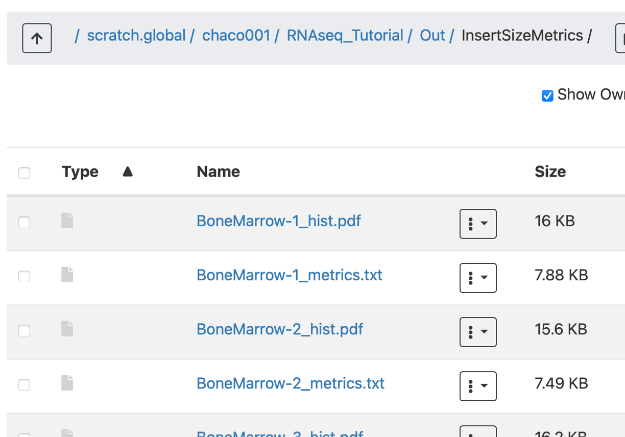
We see that there are two files for each sample, a hist.pdf file and a
metrics.txt file. The hist.pdf file contains a histogram of insert sizes
for the sample.
You should check that this distribution matches what was expected based on your molecular protocol QC. Unfortunately, for the tutorial dataset, we do not have access to such information.
The histogram is nice, but to describe the distributions in writing, we will
need textual and numerical summaries of the insert sizes. We can find these in
the metrics.txt files. This file has very long lines, so you will likely have
to use the arrow keys to
scroll side-to-side to read the information. We will not cover the meaning of
every field in this file, but you can get instructions for how to read this
file from the Picard Tools documentation:
https://broadinstitute.github.io/picard/picard-metric-definitions.html#InsertSizeMetrics
Plots Directory
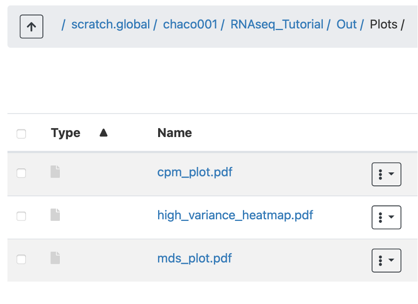
-
These are the unsupervised plots labeled with the group from group_template
-
They were made during the R analysis and are also described in the report
Logs Directory
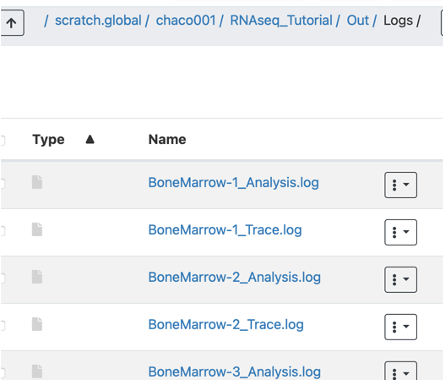
Notes:
-
There are two files per sample
-
Analysislogs can be used to see when CHURP started different sections (lines beginning with#), as well as the output from software CHURP uses. -
Tracelogs can be useful to see the progression of steps
Scheduler log files (.err, .out)
In the Out directory, a .err and .out file were made per job.
Notes:
-
If an error occurred, it should be logged in the .err file.
-
The sample name for the single-sample logs is in the first line.
-
These files aren’t critical for users to examine, but can be interested for
bookkeeping. Specifically, the .err file shows when each section started and completed.
Part 4.3: CHURP BULK_RNASeq_report.html
This report contains all of the QC metrics and analyses conducted by CHURP and is therefore likely to be the most important document to examine in detail.
To view it, download the Bulk_RNASeq_Report.html file then re-open it (just clicking is insufficient as most browsers will default to showing you the raw html).
You can also download an example here: https://pages.github.umn.edu/MSI-RIS/Tutorials/materials/rnaseq_cmd/Bulk_RNAseq_Report.html
The top of the report should look like this:
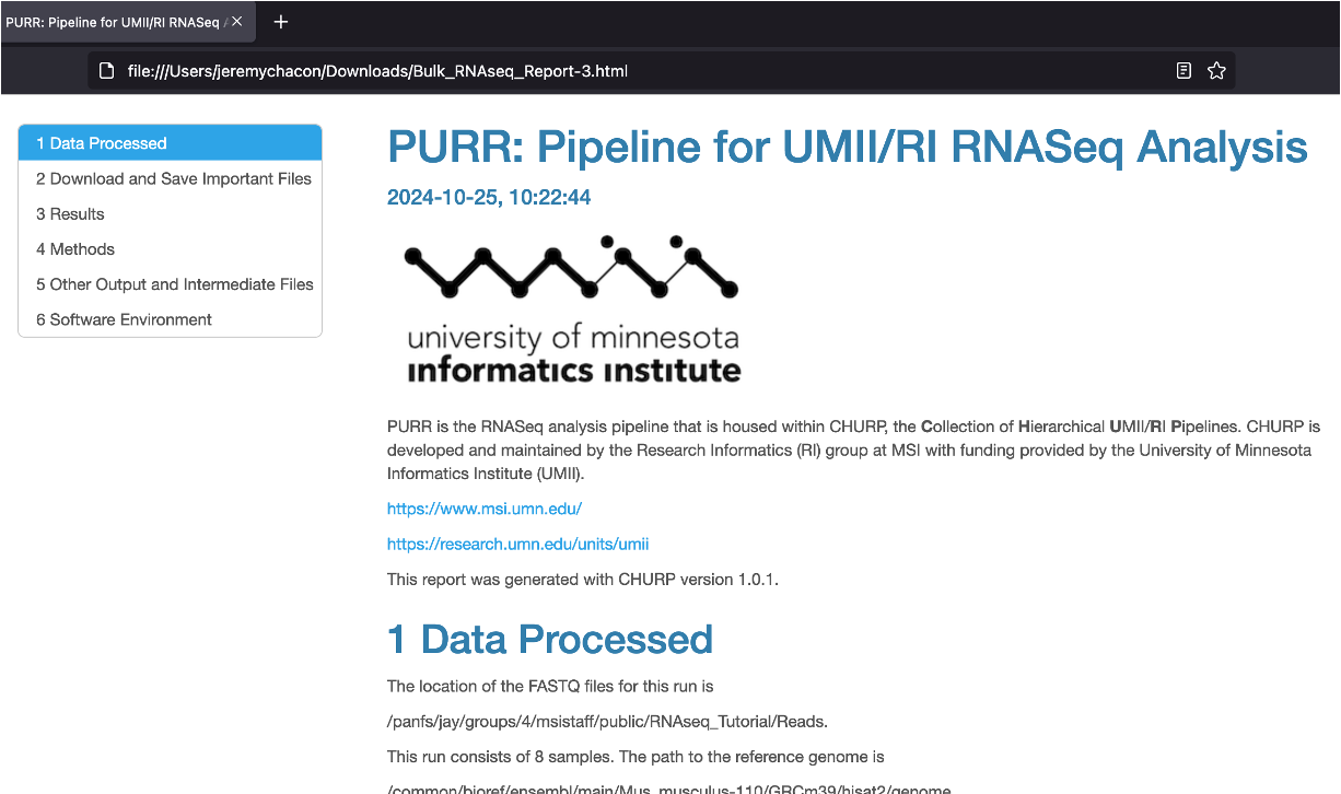
Note: The report contains downloadable files for the relative expression information (e.g. raw read counts), pipeline.sh, and samplesheet.txt.
The report itself is thoroughly self-explained. Regardless, here are some guiding questions to consider as you examine it.
- Section 1: Data Processed
- Are the sample names correct?
- Is the number of samples correct?
- Are the reference genome and annotation correct?
- Section 2.1: Read Counts
- Do any samples have extreme (high or low) values for fragment count?
- Do any samples lose a lot of reads after trimming?
- Section 2.2: Insert Size Metrics
- Do any samples have insert size distributions that do not match your expectations from a gel or BioAnalyzer?
- Section 2.3: Estimated rRNA Content
- Do any samples have very high rRNA content? Is it unexpected?
- Section 2.4: Basecall Quality
- Do any samples have very low quality overall?
- Is there a stretch of low-quality bases in the beginnings of reads?
- Section 2.5: QC Based on Mapping to Reference Genome
- Is the exon profiling efficiency close to 1? Are there samples with very low values for exon profiling efficiency?
- Are there samples with very low estimated library complexity? It should ideally be close to the number of sequenced fragments.
- Are there samples with very high sequence duplication levels?
- Do the reads look like they were sequenced from the expected strand?
- Section 3.1: Mapping Statistics
- Are there samples with very high proportions of MAPQ=0 reads?
- Are there samples that have very low mapping rates relative to others?
- Section 3.2: HISAT2 Summaries
- Are there samples with very high discordantly mapped or unmapped reads?
- Section 3.3: Feature Counts
- Are there samples with a high proportion of “Unassigned” fragments?
- Do all samples have roughly the same number of genes detected in the expression data?
- Section 4.1: Exploratory Plots*
- Do all samples have roughly the same distribution of expression values?
- What are the major groups identified in the clustering heatmap and the MDS plot? Do samples tend to cluster by group, or by some other variable?
- Section 4.2: Differential Expression Testing
- Are the groups correctly specified?
- Do the most significant DEGs make sense given your experimental design?
*: Please note that it does not necessarily indicate a failure or a quality problem if your samples do not cluster by experimental group! In fact, one of the assumptions underlying bulk RNAseq for differential gene expression analysis is that only a small number of genes (relative to all genes assayed) are truly differentially expressed across groups. The clustering plots show patterns of genome-wide gene expression, so it is not necessarily expected that experimental group is the primary axis of variation.
Part 5: Next Steps and feedback contact information
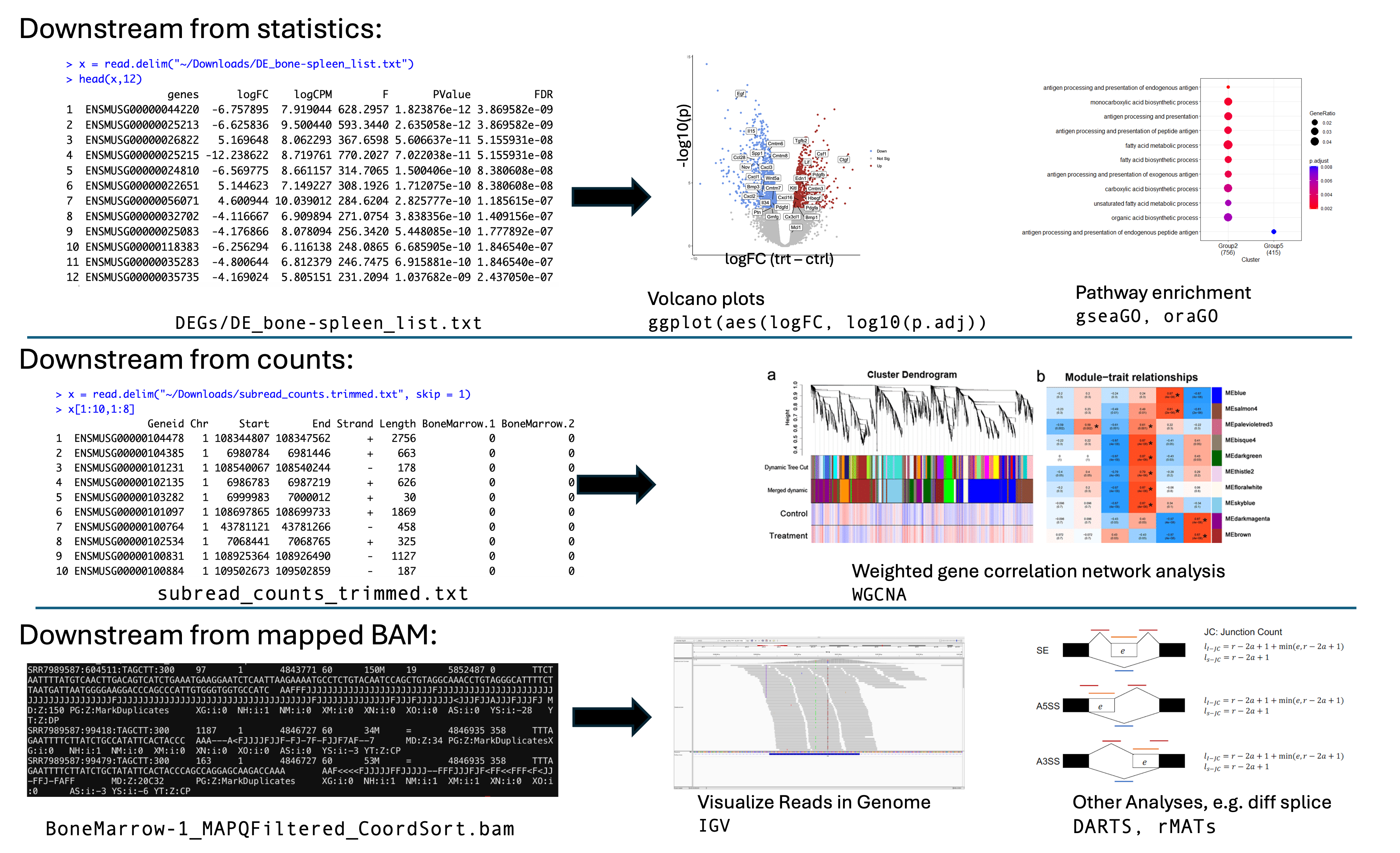
There are many other downstream analyses which can be down. This graphic summarizes some analyses and with which outputs they begin.
-
(top row) One of the most common next steps is to do pathway enrichment. We have another pipeline for that, as well as a tutorial here: https://pages.github.umn.edu/MSI-RIS/Tutorials/pathway_analysis/ It uses the DEG output as the input.
-
(middle row) Another common downstream step is to load the raw counts matrix into R and create a gene correlation matrix using WGCNA.
-
(bottom row) Many downstream options are available by starting with the BAM files, for example differential transcript abundance or differential splicing.
-
In addition, the raw fastq files could be used to, for example, create a de novo transcriptome assembly, in the case where you are working with a species lacking annotation.
FEEDBACK CONTACT
This tutorial document was prepared by Jeremy Chacón and Thomas Kono, in the RI Bioinformatics group at MSI.Please send feedback, comments, and CHURP usage questions to ribhelp [at] msi.umn.edu.
Thank you for reading this document, we hope it helps your research! What follow are a number of supplementary sections that help explain some important CHURP options as well as describe some other analyses that can be done with this sort of data. Best of luck with your research!
Supplementary Information
The information in the following sections is not part of the primary tutorial. We provide it only to discuss and illustrate issues and operations that are relevant to RNAseq analysis, but only come up in special circumstances.
Supplement 1: Custom HISAT2 Indices
In the cases where your study organism does not have a reference genome in the sections of Ensembl that we include in bioref, you will need to prepare your own index files for read mapping. You may also want to prepare a custom index if you want to restrict the genome to a specific set of regions (like we did for the tutorial), or if you have an experiment that involves a transgenic organism with a known construct transformed into it, and you want to map reads to the genome as well as the construct.
To do this, you will need at minimum the FASTA file that contains the genome sequence for your study organism. If you have the GTF annotation file, this can aid in preparing the HISAT2 index, as well. Known single nucleotide polymorphism sites (from dbSNP or VCF) can also be used.
You can find a full list of options for HISAT2 index building in their manual:
http://daehwankimlab.github.io/hisat2/manual/#the-hisat2-build-indexer
To build the index, you must be logged in to an interactive compute session:
srun -N 1 -n 1 -c 1 -t 60 --mem=4gb --tmp=2gb -p interactive --pty bash
Make sure the genome file is unzipped; the HISAT2 index builder does not take compressed FASTA input. Place this file into a directory where you would like to store the HISAT2 index files. Do the same with the GTF annotations, if you have them:
mkdir -p /home/GROUP/shared/HISAT2_Genomes/Genus_species
cp /path/to/genome.fasta.gz /home/GROUP/shared/HISAT2_Genomes/Genus_species
cp /path/to/annotations.gtf.gz /home/GROUP/shared/HISAT2_Genomes/Genus_species
gzip -d /home/GROUP/shared/HISAT2_Genomes/Genus_species/genome.fasta.gz
gzip -d /home/GROUP/shared/HISAT2_Genomes/Genus_species/annotations.gtf.gz
where GROUP is your MSI group name.
If you do not have a GTF annotation file, and instead only have a GFF
annotation file, you can convert the GFF to a GTF using the gffread utility
from the cufflinks package. This is a common scenario with reference genome
assemblies from NCBI:
module load cufflinks/2.2.1
gffread annotations.gff3 -T -o annotations.gtf
Load the HISAT2 module and navigate to the genome directory:
module load hisat2/2.1.0
cd /home/GROUP/shared/HISAT2_Genomes/Genus_species
If you want to use known splice sites to help with spliced alignment, use the
extract_splice_sites.py script that is bundled with HISAT2 to extract the
splice sites from the GTF:
extract_splice_sites.py annotations.gtf > splice_sites.txt
If you would like to use known polymorphic sites to help map reads across known
polymorphisms in your study organism, you must have either a dbSNP database
export (for humans), or a VCF with known polymorphisms. If you have a dbSNP
export, make sure the chromosome names match the genome you are using
(UCSC, Ensembl, and NCBI all have different naming conventions), then use the
hisat2_extract_snps_haplotypes_UCSC.py script to extract them:
hisat2_extract_snps_haplotypes_UCSC.py genome.fasta dbSNP.txt hisat2_snps
If you have a VCF, you can use the hisat2_extract_snps_haplotypes_VCF.py
script to do the same thing:
hisat2_extract_snps_haplotypes_VCF.py genome.fasta SNPs.vcf hisat2_snps
Then, you are ready to build the genome index. This step should be done as a
non-interactive batch job. It requires a lot of time and memory. For example,
to build the human genome index with known splice sites and known
polymorphisms, it takes at least several hours and about 200GB of RAM. The
script would look something like the following. Remove the option for --ss if
you do not have known splice sites, and remove options for --snp and
--haplotype if you do not have known polymorphic sites. Note that you may
have to adjust the resource requests if you experience walltime errors or
out-of-memory errors, and use your email address instead of
YOUR_INTERNET_ID:
#!/bin/bash
#SBATCH -N 1
#SBATCH -n 1
#SBATCH -c 16
#SBATCH --mem=500gb
#SBATCH -t 36:00:00
#SBATCH --mail-type=BEGIN,END,FAIL
#SBATCH --mail-user=YOUR_INTERNET_ID@umn.edu
#SBATCH -p ram1t
#SBATCH -e HISAT2_Build_%j.err
#SBATCH -o HISAT2_Build_%j.out

module load hisat2/2.1.0

cd /home/GROUP/shared/HISAT2_Genomes/Genus_species
hisat2-build -f \
    -p 16 \
    --ss splice_sites.txt \
    --snp hisat2_snps.snp \
    --haplotype hisat2_snps.haplotype \
    genome.fasta \
    hisat2_genome_idx
Submit the job with sbatch and wait for it to finish. There will eventually be
eight files that make up the genome index, and they must all be present in the
same directory and have the same prefix. The name of your genome index will
then be hisat2_genome_idx, and you can use this with the -x option to
CHURP’s bulk RNAseq workflow:
...
-x /home/GROUP/shared/HISAT2_Genomes/Genus_species/hisat2_genome_idx
...
You can find a full list of options for HISAT2 index building in their manual:
http://daehwankimlab.github.io/hisat2/manual/#the-hisat2-build-indexer
Supplement 2: Customizing CHURP Behavior
We try to provide “sensible defaults” for CHURP’s behavior, but as with any analytical workflow, there exist datasets that require adjustment to the parameters. Most of the time, these cases can be addressed by adjusting the options to the read mapping software or the trimming software. In Supplement 3, we provide instructions for adjusting the expression quantification if you need a different type of expression analysis than the default gene-level expression.
Supplement 2.1: Custom HISAT2 Options
CHURP provides the --hisat2-opts option for adjusting the HISAT2 options. This
is required when handling datasets that do not match the “default” dataset that
CHURP expects. For example, if your paired-end reads are “interleaved” - R1 and
R2 are contained in the same file rather than in separate files. Another case
might be if you are analyzing a dataset with different quality score encodings:
at the time of this writing, Illumina quality scores are “PHRED+33” but older
datasets are “PHRED+64.”
Wikipedia has a good description of the various types of quality score encodings
that you may encounter in FASTQ format:
https://en.wikipedia.org/wiki/FASTQ_format#Quality
Data that is generated contemporary to this writing will be in “Sanger” scale, with “PHRED+33” encoding.
You may additionally want to change how HISAT2 handles discordant read pairs or
read pairs that fail to map to the genome. All of these options are available
to adjustment! Please see the HISAT2 manual for the full range of options that
you can provide:
http://daehwankimlab.github.io/hisat2/manual/
The default options that we supply for HISAT2 are the following:
-p 6(use 6 cores, adjustable with the--ppnoption to CHURP, too)--no-mixed(do not map discordant pairs as separate single-reads)--new-summary(print machine-friendly summary)
To specify custom HISAT2 options, you must pass it as a quoted string. This is because CHURP unfortunately tries to treat the options meant for HISAT2 as its own, and throws errors. For example, the default options defined above would be passed as follows:
...
--hisat2-opts="-p 6 --no-mixed --new-summary"
...
Any adjustment to the HISAT2 options with --hisat2-opts requires that you
set all of the HISAT2 options. For example, if you are handling data that
has “PHRED+64” quality scores, you would specify --phred64, but you will then
also have to specify the multithreading options and pair-handling options:
...
---hisat2-opts="-p 6 --phred64 --no-mixed"
...
We require this because it is impossible for us to verify every possible combination of HISAT2 options. It is also possible that the custom HISAT2 options are incompatible with downstream expression quantification routines. If you encounter errors while providing custom HISAT2 options, you must troubleshoot the errors independently.
Supplement 2.2: Custom Trimmomatic Options
CHURP also provides the --trimmomatic-opts option for adjusting the behavior
of Trimmomatic. This would be required when handling data that have
non-standard adapter sequences or if your data have a quality score encoding
that is not “PHRED+33.”
The default options string that we pass to Trimmomatic is below:
ILLUMINACLIP:4:15:7:2:true LEADING:3 TRAILING:3 SLIDINGWINDOW:4:15 MINLEN:18
Which performs the following steps:
ILLUMINACLIP:4:15:7:2:true: trim the standard Illumina adapters, allowing up to 4 mismatches, a palindrome clip threshold of 15 (when “read-through” into the adapter is detected in short fragments), minimum palindrome adapter length of 7, and keep both reads in the pair if a palindrome is detected.LEADING:3: trim bases from the start of the read if they have quality scores lower than 3.TRAILING:3: trim bases from the end of the read if they have quality scores lower than 3.SLIDINGWINDOW:4:15: divide the read into 4-base wide sliding windows, removing windows where the mean quality score is below 15.MINLEN:18: remove read if it is shorter than 18bp after the previous trimming steps have been applied.
Like with the custom HISAT2 options, these must be passed as a quoted string. The default options would look like the following:
...
--trimmomatic-opts="ILLUMINACLIP:/path/to/adapters.fa:4:15:7:2:true LEADING:3 TRAILING:3 SLIDINGWINDOW:4:15 MINLEN:18"
...
Additionally, any adjustment to the Trimmomatic options requires that you
specify the entire options string. The only exception is adding a
HEADCROP operation, which can be done through CHURP by adding the
--headcrop option (we provide this for handling the Takara Bio library
preparation protocols).
Please see the Trimmomatic homepage to view the manual that gives the full range
of options that are supported:
http://www.usadellab.org/cms/?page=trimmomatic
Supplement 3: Transcript-level Analyses
By default, CHURP performs expression quantification at the gene feature level. This is the feature level that is targeted by most bulk RNAseq experiments and the feature level at which expression is most confidently measured. If you would like to instead measure transcript (isoform) feature expression, you will have to take special care with the molecular protocol and sequencing (data collection) as well as the downstream analytical workflow.
We cannot provide nearly complete scripts like we can with Supplement 1 because transcript-level analyses are highly specific to each study. Both the experimental design and the idiosyncrasies of the study system affect how the analysis is carried out. We instead provide points to consider when performing a transcript-level analysis. Of course, if you work in a research system that does not have alternative splicing, then this does not apply!
Supplement 3.1: Data Collection Considerations
Measuring isoform expression requires that you be able to distinguish the transcripts based on their splicing junctions or untranslated sequences. Additionally, detecting isoforms that have low expression requires deeper sequencing than detecting gene-level expression. You may also be interested in conditionally-expressed isoforms (tissue-specific, disease-specific, etc), which requires special experimental designs.
Unfortunately, we cannot provide general recommendations for sequencing depth nor sampling strategies to capture these cases. You should have a good sense of the “dynamics” of the genome of your study species - the distribution of the number of annotated isoforms for each gene model and the circumstances under which they are expressed will help to guide your experiments. The moments of that distribution will also guide you in sequencing depth; for example, if there are 4 isoforms per gene on average, you should expect to collect at least 4 times as much sequence data as for a gene-level experiment. The real number will be higher because not every isoform is expressed at the same level.
For human or mouse RNAseq experiments, this means you will need to collect at least 100 million read pairs (fragments) per sample for isoform level expression studies. If you want to assay the rare isoforms, then you likely will need to collect at least 200 million read pairs per sample. You may be able to use shorter read length to offset the cost of collecting so many reads, but that depends on the nature of the genes in your study system.
Supplement 3.2: Analytical Workflow Considerations
The read QC and trimming portions of the workflow can proceed as they would with CHURP. However, obtaining accurate transcript-level counts requires deviating from the CHURP workflow at the read mapping step. Instead of mapping read pairs to the reference genome with HISAT2, you should use a tool like RSEM (RNASeq by Expectation Maximization; Li and Dewey 2011; https://bmcbioinformatics.biomedcentral.com/articles/10.1186/1471-2105-12-323) to perform transcript quantification. The reason you need to change the read mapping workflow is that RSEM can estimate the transcript of origin for each fragment, while HISAT2 cannot. Because the multiple transcripts from a gene model are highly overlapping, the mapping-then-counting approach with HISAT2 and featureCounts cannot accurately estimate expression of the isoforms.
Please see the RSEM GitHub page (https://github.com/deweylab/RSEM#readme-for-rsem) for usage information and examples that show how to use it.
If you are confident that the reads from your experimental samples are very similar to the reference genome (less than 0.1% different at the nucleotide level), then you can use tools like Salmon (Patro et al. 2017; https://www.nature.com/articles/nmeth.4197) or Kallisto (Bray et al. 2016; https://www.nature.com/articles/nbt.3519) to estimate transcript abundances from reads. These two methods rely on very high similarity between the reads the reference genome, however, so we do not recommend them for general-purpose RNAseq, where you expect sequence differences between the experimental samples and the reference genome.
See the Salmon documentation (https://salmon.readthedocs.io/en/latest/) and the Kallisto documentation (https://pachterlab.github.io/kallisto/manual) for instructions on how to use their software to estimate transcript abundance.
All of RSEM, Salmon, and Kallisto are available on MSI systems as software modules:
module avail rsem
-------------------------------- /panfs/roc/soft/modulefiles.common --------------------------------
rsem/1.3.0
module avail salmon
--------------------------------- /panfs/roc/soft/modulefiles.hpc ----------------------------------
salmon/0.14.1  salmon/1.2.1
module avail kallisto
-------------------------------- /panfs/roc/soft/modulefiles.common --------------------------------
kallisto/0.43.1  kallisto/0.46.2
Transcript abundance estimates from the above-mentioned tools will not work with the same routines for differential expression testing as gene-level counts data. Gene-level expression is count-based (i.e., the data are integers), while transcript abundances are often reported in “TPM” (transcripts per million) values and “estimated counts” values. You can use the “estimated counts” values in a differential expression workflow built for analyzing counts data, like those in DESeq2 or EdgeR. If you use the TPM values, you can use a program like Sleuth (Pimentel et al. 2017; https://www.nature.com/articles/nmeth.4324; https://github.com/pachterlab/sleuth) to perform differential expression analysis.
Supplement 4: CPM, TPM, FPKM, RPKM, etc
RNAseq expression analyses are sometimes performed with normalized relative expression values rather than with raw fragment counts like we have done in this tutorial. Some analyses like coexpression network analyses, require normalized relative expression values rather than fragment counts.
Differential gene expression analyses should always be done with the raw
fragment counts because the software packages that perform these analyses have
statistical routines to properly model the distribution of expression values
from fragment count data. The R packages discussed in this tutorial(edgeR and
DESeq2) additionally perform robust cross-sample normalization, which none of
the units described here will incorporate. These expression values should only
be used as auxiliary to the results from the actual differential gene
expression tests.
These units are also specific to the experiment or sequencing run. They are NOT comparable across experiments because they are very sensitive to the composition of the libraries. To properly analyze data from multiple experiments, you must take a meta-analysis approach; consult with a statistician!
Normalized relative expression values are useful for comparing genes or samples when there are differences in sequencing depth and gene length. For example, if you were to compare the fragment counts of a single gene across multiple samples, then both gene expression variation and sequencing depth variation will contribute to the fragment counts differences. On a related note, if you were to compare the fragment counts of different genes in the same sample (e.g., to check if knock-down of one gene leads to other gene expression responses), then both gene expression response and gene length differences will contribute to counts differences. This is because longer genes and transcripts have a larger “sequencing target” than shorter genes and transcripts. If two genes have the same transcript abundance, then the longer gene will have higher fragment counts simply because there is a higher representation of its transcript in the sequencing library.
One common relative expression value is normalized counts per million(CPM). To
calculate CPM, first sum the fragment counts from all genes, and divide the sum
by 1,000,000: this is the “per million” scaling factor. Then, for each gene,
divide its fragment count by the scaling factor. This value is useful for
comparing the same gene across samples because it accounts for sequencing
depth variation. It is not useful for comparing different genes within the
same sample because it does not account for gene length differences.
Specifically with EdgeR, the values are output on the log2 scale, and
a “pseudocount” is added to the raw counts value before normalizing by library
size to avoid calculating log2(0).
Another common relative expression value is transcripts per kilobase-million
(TPM). This value is proportional to transcript relative abundance within a
single sequencing library. For each gene or transcript, calculate a “counts per
kilobase” value, which is the fragment count divided by the length of the
gene/transcript in kilobases (length / 1000). Sum the “counts per kilobase”
values across all genes or transcripts and divide by 1,000,000: this is
the “per million” scaling factor. Divide each gene or transcript’s “counts per
kilobase” value by the scaling factor. One feature of TPM values is that the
sum of all per-feature TPM values will be equal across samples (much like
describing concentration values in a mixture with ppm). However, it is
sensitive to library composition differences among samples, so it should not be
used to compare relative expression of a gene between samples.
Really, RPKM and FPKM should just be abandoned. We include them here just because some researchers still use them (and older publications report them).
Older units like reads per kilobase per million (RPKM; single-read data)
and fragments per kilobase per million (FPKM; paired-end and single-read
data) are very similar in spirit to TPM. The main difference is that TPM
normalizes first by the gene or transcript length, then by sequencing depth,
while RPKM and FPKM normalize first by sequencing depth then by gene or
transcript length. While this difference seems minor, RPKM and FPKM do not have
the property that the sum of expression values is the same for each sample.
Thus, it is not possible to interpret FPKM or RPKM differences as proportional
differences in transcript abundance. It is also worth noting that Cufflinks
includes some probabilistic read mapping parameters in its FPKM calculations,
so the FPKM values obtained from Cufflinks will be different than if you
calculate them via the formula as written.
This was once a topic of much discussion, and you can read a nice summary of
various expression values and their merits and weaknesses here:
https://haroldpimentel.wordpress.com/2014/05/08/what-the-fpkm-a-review-rna-seq-expression-units/
Supplement 5: Depositing Data into GEO
After you have finished analyzing your experiment and interpreting the results, you will likely want to publish your findings. Many journals require that your raw reads and processed expression data be made available in public repositories, like NCBI’s Gene Expression Omnibus (GEO). GEO accession numbers may also be required during peer review so it is important to note this section as you are preparing your manuscript. GEO can also place a hold or embargo on your data until publication, so your data can remain private until you decide to release it.
Submitting your raw and processed data to GEO will make it available in both GEO and NCBI’s Sequence Read Archive (SRA).
GEO says it can take up to five (5) business days to issue accession numbers for your dataset. Please plan accordingly!
The lab who is publishing the study should be the ones to manage the GEO submission. The submission process requires detailed knowledge of the experimental design, so the people who performed the experiment should be the ones to submit the data.
Required Data/Information
GEO requires both data and metadata for your submission. It is important that your metadata be complete and informative; these are what make datasets in public repositories useful.
You will also need to log in to GEO (requires an NCBI account) to initiate the submission process. You can initiate the submission process here: https://www.ncbi.nlm.nih.gov/geo/submitter/
Do make a note of the FTP URL and credentials (FTP username and FTP password) for later. You will need these for data transfer.
Required Data
The data required are the raw demultiplexed FASTQ files and the processed
relative expression data. If you collected your data through the UMGC, then the
raw data are the FASTQ files that are included in the data release from UMGC.
If you processed your data through CHURP, then the cpm_list.txt normalized
relative expression matrix and subread_counts.txt raw read counts matrix have
the expression data that are required. Additionally, the MD5 sums for verifying
file integrity are required; we will go over this in a later section.
The metadata required are given in the GEO submission template linked below
(Example 1 is for ChIP-seq, and example 2 is for RNAseq):
https://www.ncbi.nlm.nih.gov/geo/info/seq.html#metadata
The required information includes:
- Project title
- Project summary
- Short description of the experimental design
- Contributors’ names
- Study organism, including genotype/strain if applicable
- Sample characteristics:
- Human-readable sample name
- Experimental treatment or condition
- Age (if applicable)
- Sex (if applicable)
- Tissue/organ (if applicable)
- Other characteristics that are important for the experimental design
- Molecule type (e.g., messenger RNA)
- Sample rearing/handling protocol:
- Growth conditions (if applicable)
- Experimental treatment protocol (if applicable)
- Molecular protocol information:
- Nucleic acid extraction protocol
- Library preparation protocol
- Data processing protocol*
*: This tutorial covers the data processing protocol! The read trimming, read mapping, alignment filtering, expression quantification, and expression normalization steps described in this tutorial describe the steps taken to handle the data.
Calculating MD5 Sums
The MD5 sums are required for all raw and processed data that will be deposited into GEO. These are strings that can be used to verify file integrity in non-cryptographic situations, e.g., to make sure the file you are using is not unintentionally corrupted.
If you are working on a funded collaboration with RI Bioinformatics, we can perform the MD5 sum calculation step for you!
You can perform this calculation on MSI’s compute servers. First, request an interactive compute session:
srun -N 1 -n 1 -c 1 --mem=2gb -t 4:00:00 -p interactive --pty bash -l
Once you have an interactive session, navigate to where your raw reads are stored. For this example, we will use the tutorial reads:
cd /home/msistaff/public/RNAseq_Tutorial/Reads
Then use the md5sum command to generate the checksums and write them to a
file:
md5sum *.fastq.gz > ~/geo_submission_md5sums.txt
You can verify they were properly generated by passing the -c option to the
md5sum command:
md5sum -c ~/geo_submission_md5sums.txt
BoneMarrow-1_S23_R1_001.fastq.gz: OK
BoneMarrow-1_S23_R2_001.fastq.gz: OK
BoneMarrow-2_S21_R1_001.fastq.gz: OK
BoneMarrow-2_S21_R2_001.fastq.gz: OK
BoneMarrow-3_S19_R1_001.fastq.gz: OK
BoneMarrow-3_S19_R2_001.fastq.gz: OK
BoneMarrow-4_S17_R1_001.fastq.gz: OK
BoneMarrow-4_S17_R2_001.fastq.gz: OK
Spleen-1_S31_R1_001.fastq.gz: OK
Spleen-1_S31_R2_001.fastq.gz: OK
Spleen-2_S29_R1_001.fastq.gz: OK
Spleen-2_S29_R2_001.fastq.gz: OK
Spleen-3_S27_R1_001.fastq.gz: OK
Spleen-3_S27_R2_001.fastq.gz: OK
Spleen-4_S25_R1_001.fastq.gz: OK
Spleen-4_S25_R2_001.fastq.gz: OK
Every file passes! The contents of the file are pasted below. The first column is the MD5 sum and the second column is the filename. The strings listed in the first column are what you would enter into your GEO submission sheet:
ee99e5e5262a0131451460845197378d  BoneMarrow-1_S23_R1_001.fastq.gz
b7ad1164d691010b397942cca8f6fc39  BoneMarrow-1_S23_R2_001.fastq.gz
614195cfc82221d93861ec265c627d29  BoneMarrow-2_S21_R1_001.fastq.gz
b49dc13ae696334525daa0b91fb1bda6  BoneMarrow-2_S21_R2_001.fastq.gz
ae2071b5c9f7e966a01e8c73779de204  BoneMarrow-3_S19_R1_001.fastq.gz
2208e126306480767354b135e9d3475b  BoneMarrow-3_S19_R2_001.fastq.gz
7c5168e84f55ba2bf6072ff2bbdb855b  BoneMarrow-4_S17_R1_001.fastq.gz
de2a0f9b67a61444cbd6d2bdd9840263  BoneMarrow-4_S17_R2_001.fastq.gz
e7900214eef5872f7797656933b32182  Spleen-1_S31_R1_001.fastq.gz
2d9fde82c0dc57fff855897eac1bc6b2  Spleen-1_S31_R2_001.fastq.gz
5d17363dc573b37c2c23c9acc592a200  Spleen-2_S29_R1_001.fastq.gz
9112d0acbb1f7eace510f00e72ddd828  Spleen-2_S29_R2_001.fastq.gz
821f8d7ed25d6e37a8a5bd0123193833  Spleen-3_S27_R1_001.fastq.gz
eebe5f6e30ab1fafd38426e20887a09e  Spleen-3_S27_R2_001.fastq.gz
b20468603ce262c38f5378e7feb580e8  Spleen-4_S25_R1_001.fastq.gz
5ba0d064a1bc09e7f38138f4fe55dec3  Spleen-4_S25_R2_001.fastq.gz
The process is the same for the raw read counts matrix and the normalized expression matrix.
Uploading Data to GEO
Now that you have the MD5 sums calculated and entered into your submission spreadsheet, you can upload the data files to GEO.
If you are working on a funded collaboration with RI Bioinformatics, we can upload the data for you, too!
If your data are larger than 1 terabyte (TB, 1000 GB) in volume, you must contact GEO and wait for a response from them before uploading the data.
Again, we can do this from the MSI compute node. First request an interactive compute session:
srun -N 1 -n 1 -c 1 --mem=2gb -t 4:00:00 -p interactive --pty bash -l
Then, navigate to the directory where your raw data are stored. This example has the tutorial dataset, but you should use your raw FASTQ folder:
cd /home/msistaff/public/RNAseq_Tutorial/Reads
We will then use an FTP client (lftp) to connect to the GEO upload location
and put the files there. Fetch the FTP address and username and password that
were provided to you by GEO. Use these to connect to the server, make a
directory for your data uploads, and then upload the files. Note that there are
no spaces between the USERNAME and PASSWORD in the following command, just
a comma:
lftp -u USERNAME,PASSWORD ftp://ftp.ncbi.../uploads/
lftp ftp.ncbi.nlm.nih.gov:/uploads> mkdir my_submission
lftp ftp.ncbi.nlm.nih.gov:/uploads> cd my_submission
lftp ftp.ncbi.nlm.nih.gov:/uploads/my_submission> mput *.fastq.gz
Note that the lftp prompt shows you which server you are connected to and
which directory you are in. Once these files are uploaded, you can use the
lcd command to navigate to where your raw read counts and normalized
expression matrices are stored. Upload these, too. Again, we will use the
tutorial directory, but you should use your real data:
lftp ftp.ncbi.nlm.nih.gov:/uploads/my_submission> lcd /scratch.global/konox006/RNAseq_Tutorial/Out/Counts
lftp ftp.ncbi.nlm.nih.gov:/uploads/my_submission> put subread_counts.txt
lftp ftp.ncbi.nlm.nih.gov:/uploads/my_submission> put cpm_list.txt
lftp ftp.ncbi.nlm.nih.gov:/uploads/my_submission> bye
The bye command closes the FTP connection. Note that your terminal may print
more output messages than what I have listed here. So long as you do not see
errors, your command worked.
Using your favorite desktop FTP client (OSX Finder or Windows Explorer both work for this; if you are on Linux, then you can find an FTP client on your own), transfer your GEO metadata spreadsheet into the submission directory as well. You can transfer it through MSI servers via the same process above if you are more comfortable with it, but I find it more convenient to transfer from my workstation.
Notifying GEO of File Upload
Once your raw data, processed data, and metadata spreadsheet are uploaded, you
can go to this link to notify GEO that your files are ready for review:
https://submit.ncbi.nlm.nih.gov/geo/submission/
If you have a funded collaboration with RI Bioinformatics, then we can do this step for you!
This form will require the following information:
- FTP directory where the data and metadata are deposited (in this example
/uploads/my_submission) - List of filenames that were uploaded
- Release date of the data (can be in the future for data to be held privately during review)
- Optional information:
- NCBI account name for someone who should be associated with the study, e.g., the PI of the study if you are uploading on behalf of them
- Explanations of incomplete data
Once you submit the form, wait for a response from GEO. They will contact you if any of the metadata are incomplete or if any files were corrupted during upload. Once everything checks out, they will send you a link to the study that you can include for peer review.
Glossary of Terms
This section describes the specialized terms that we use in this tutorial. I have tried to point out terms that may be used differently from how I use them in this tutorial.
Molecular Biology (Wet Bench) Terms
- (Sequencing) Adapter: Short nucleotide oligomers that are ligated to the 5′ and 3′ ends of a fragment in a sequencing library. These are non-biological sequences and are complementary to the oligomers that are present in the flow-cell for sequencing.
- Insert: A specific stretch of nucleic acid that retained for sequencing during library preparation. It is called an “insert” because it is “inserted” between two sequencing adapters. One characteristic of a sequencing library is its insert size distribution - the distribution of lengths of the insert sequences.
- Fragment: A molecule in the sequencing library that consists of an insert
between two adapters:
Adapter-Insert-Adapter. - Library: A collection of nucleic acid molecules that represents the sample organism that you wish to study. For RNAseq, it is usually a collection of cDNA (complementary DNA) sequences synthesized from RNA molecules.
- Library Preparation: The protocol that converts an extracted sample of nucleic acid into a sequencing library, read to run on the instrument. Various library preparation protocols exist, so it is important to know the details of the protocols your experiments are using. The details of the protocol do affect how your data should be handled, in particular, the sequencing adapters, strand-specificity, and ribosomal RNA depletion method must be known.
- Sequencing Read: A string of nucleotide bases identified by the sequencing instrument. The nucleotide bases are derived from the sequence of the inserts of the sequencing library.
Bioinformatic Terms
- Base Quality: A numerical value associated with each nucleotide base call generated by a sequencing instrument. The number is proportional to the probability that the base call is correct.
- Coverage: The degree to which a particular sequence (gene, e.g.) is represented by reads. Higher coverage means more of the sequence is represented in the data.
- Depth: The number of times a particular nucleotide position has been seen in sequencing reads. Higher depth means the nucleotide has been read more times and thus typically has less uncertainty. Note that some people use “coverage” or “fold coverage” to refer to this definition of “depth.”
- Gene Annotation: (Noun) The assignment of regions of a reference genome to gene models. The assignments are stored in “annotation files” with formats such as GTF or GFF3. A gene annotation file must only be used with its accompanying reference genome file.
- Mapping: A process by which short sequencing reads are compared to a reference genome to identify where they originated. This is the process that is used in inferring the relative abundance of transcripts in a RNA extraction. I distinguish mapping from alignment in that alignment is used to identify homologous sequences (rather than simply identifying a genomic position) and uses different algorithms from mapping. Some people use “mapping” and “alignment” interchangeably.
- Mapping Quality: A numerical value that describes the confidence with which the mapping position is known. Higher values indicate higher confidence. Each mapped read (or read pair) will have a mapping quality value associated with it.
- Normalization: A technique for adjusting the relative gene expression values across samples to account for variation in library size.
- (Raw) Counts Matrix: A matrix of integers describing the assignment of mapped reads to annotated gene models across multiple samples. The raw counts matrix is the input for a differential gene expression analysis.
- Reference Genome: A string of nucleotides that describes the genome of a given species. Sequencing reads are mapped against a reference genome, and gene expression is quantified using the accompanying gene annotation file.